Table of contents

1. (BRIEF) INTRODUCTION
2. FORMALIZATION OF SCENARIOS AND GENERATION OF THE TRAINING SET
5. RUNNING (EXAMPLE) DATASET TREATMENTS USING THE GRAPHIC USER INTERFACE (GUI)
6. PERFORMING RANDOM FOREST ANALYSES
7. KEY FILES

USER MANUAL for DIYABC Random Forest v1.0

- 23th of March 2021 -

François-David Collin ^1,*, Ghislain Durif ^1,*, Louis Raynal ¹, Eric Lombaert ², Mathieu Gautier ³, Renaud Vitalis ³, Jean-Michel Marin ^1,&, Arnaud Estoup ^3,&

¹ IMAG, Univ Montpellier, CNRS, UMR 5149, Montpellier, France

² ISA, INRAE, CNRS, Univ Côte d’Azur, Sophia Antipolis, France

³ CBGP, Univ Montpellier, CIRAD, INRAE, Institut Agro, IRD, Montpellier, France

^* Equal contribution (F-D.C.: computation part of the program; S.D.: interface part of the program)

^& These authors are joint senior authors on this work

Corresponding authors:

Arnaud Estoup. E-mail: arnaud.estoup@.inrae.fr

Francois-David.Collin: Francois-David.Collin@umontpellier.fr

Ghislain Durif: ghislain.durif@umontpellier.fr

Warning: You might want to activate the option “Navigation panel” (accessible through the “Display” tab) after opening the present manual file under Word. This navigation panel, visible on the left size of the document once activated, will allow you reaching directly through simple click actions the different sections and sub-sections described below. You can navigate just by directly clicking on the titles of the content below when using the pdf format of the present document.

1. (BRIEF) INTRODUCTION

1.1 General context

Simulation-based methods such as Approximate Bayesian Computation (ABC) are well adapted to the analysis of complex models of populations and species genetic history (Beaumont 2010). In this context, supervised machine learning (SML) methods provide attractive statistical solutions to conduct efficient inferences about both scenario choice and parameter estimation (Schrider & Kern 2018). The Random Forest methodology (RF) is a powerful ensemble of SML algorithms used for both classification and/or regression problems (Breiman 2001). RF allows conducting inferences at a lower computational cost than ABC, without preliminary selection of the relevant components of the ABC summary statistics, and bypassing the derivation of ABC tolerance levels (Pudlo et al. 2018; Raynal et al. 2019). We have implemented a set of RF algorithms to process inferences using simulated datasets generated from an extended version of the population genetic simulator implemented in DIYABC v2.1.0 (Cornuet et al. 2014). The resulting computer package, named DIYABC Random Forest v1.0, integrates two functionalities into a user-friendly interface: the simulation under custom evolutionary scenarios of different types of molecular data (microsatellites, DNA sequences or SNPs – including traditional IndSeq and more recent PoolSeq SNP data) and RF treatments including statistical tools to evaluate the power and accuracy of inferences (Collin et al. 2020). Because of the properties inherent of the implemented RF methods and the large feature vector (including various summary statistics and their linear combinations) available for SNP data, DIYABC Random Forest v1.0 can efficiently contribute to the analysis of large-size SNP (and other molecular markers) datasets to make inferences about complex population genetic histories.

1.2 How to cite the program DIYABC Random Forest v1.0

Collin F-D, Durif G, Raynal L, Lombaert E, Gautier M, Vitalis R, Marin J-M, Estoup A (2021) DIYABC Random Forest v1.0: extending approximate Bayesian computation with supervised machine learning to infer demographic history from genetic polymorphisms. Molecular Ecology Resources. DOI: 10.22541/au.159480722.26357192

1.3 Web site

https://diyabc.github.io.

You can get from this github site the executable files for different operating systems, the latest version of this manual document, as well as examples of DIYABC Random Forest analyses for different types of markers.

1.4. System requirements, installing and launching the program

The software DIYABC Random Forest (hereafter DIYABC-RF) v1.0 is composed of three parts: the dataset simulator, the Random Forest inference engine and the graphical user interface. The whole is packaged as a standalone and user-friendly graphical application named DIYABC-RF GUI and available at https://diyabc.github.io. The different developer and user manuals for each component of the software are available on the same website. DIYABC-RF is a multithreaded software which can be run on three operating systems: GNU/Linux, Microsoft Windows and MacOS. The program can be used through a modern and user-friendly graphical interface designed as an R shiny application (Chang et al. 2019). For a fluid and simplified user experience, this interface is available through a standalone application, which does not require installing R or any dependencies and hence can be used independently. The application is also implemented in an R package providing a standard shiny web application (with the same graphical interface) that can be run locally as any shiny application, or hosted as a web service to provide a DIYABC-RF server for multiple users.
To install and run the program, please check the instructions available on the website https://diyabc.github.io/
Minimum 4GB of RAM; 6GB of RAM recommended
From 1 to 10 GB free disk space for each DIYABC-RF project depending on the project configuration and the number of simulated datasets recorded in the training set file (reftableRF.bin file).

1.5 Acknowledgements

We thank Pierre Pudlo for useful discussions and Jean-Marie Cornuet for computer code expertise at the onset of the ABC Random Forest project. We also thank several “beta-users”, especially XXXNAMEXXX, who tested the software DIYABC Random Forest v1.0 with their data. This work was supported by funds from the French Agence National pour la Recherche (ANR projects SWING and GANDHI), the INRAE scientific division SPE (AAP-SPE 2016), and the LabEx NUMEV (NUMEV, ANR10-LABX-20).

2. FORMALIZATION OF SCENARIOS AND GENERATION OF THE TRAINING SET

2.1 Basic notions

Before processing Random Forest analyses, one need to generate a training set which corresponds to the so called reference table in a standard ABC framework (Cornuet et al. 2014 and see the associated program DIYABC v2.1.0). The datasets composing the training set can be simulated under different models (hereafter referred to as scenarios) and samples (i.e. nb of markers and sampled individuals) configurations, using parameter values drawn from prior distributions. Each resulting dataset is summarized using a set of descriptive statistics. Scenarios and prior distributions are formalized in the main pipeline of the software DIYABC-RF and summary statistics are computed using the “Training set simulation” module of the main pipeline of DIYABC-RF, which essentially corresponds to an extended version of the population genetics simulator implemented in DIYABC v2.1.0 (Cornuet et al. 2014). As in the latter program, DIYABC-RF allows considering complex population histories including any combination of population divergence events, symmetrical or asymmetrical admixture events (but not any continuous gene flow between populations) and changes in past population size, with population samples potentially collected at different times. Statistical analysis based on Random Forest algorithms of an observed dataset using a given training set are computed using the “Random Forest Analysis” module of the main pipeline of DIYABC-RF.

2.2 Main features of algorithms for data simulation

The ABC part of DIYABC-RF is a simulation-based method. Data simulation is based on the Wright-Fisher model. It consists in generating the genealogy of all sampled genes until their most recent common ancestor using (backward in time) coalescence theory. This begins by randomly drawing a complete set of parameters from their own prior distributions and that satisfy all imposed conditions. Then, once events have been ordered by increasing times, a sequence of actions is constructed. If there is more than one locus, the same sequence of actions is used for all successive loci.

Possible actions fall into four categories:

- adding a sample to a population = Add as many gene lineages to the population as there are genes in the sample.

- merge two populations = Move the lineages of the second population into the first population.

- split between two populations = Distribute the lineages of the admixed population among the two parental populations according to the admixture rate.

- coalesce and mutate lineages within a population = There are two possibilities here, depending on whether the population is terminal or not. We call terminal the population including the most recent common ancestor of the whole genealogy. In a terminal population, coalescences and mutations stop when the MRCA is reached whereas in a non-terminal population, coalescence and mutations stop when the upper (most ancient) limit is reached. In the latter case, coalescences can stop before the upper limit is reached because there remains a single lineage, but this single remaining lineage can still mutate.

Two different coalescence algorithms are implemented: a generation by generation simulation or a continuous time simulation. The choice, automatically performed by the program, is based on an empirical criterion which ensures that the continuous time algorithm is chosen whenever it is faster than generation by generation while keeping the relative error on the coalescence rate below 5% (see Cornuet et al. 2008 for a description of this criterion). In any case, a coalescent tree is generated over all sampled genes.

Then the mutational simulation process diverges depending on the type of markers: for microsatellite or DNA sequence loci, mutations are distributed over the branches according to a Poisson process whereas for SNP loci, one mutation is applied to a single branch of the coalescent tree, this branch being drawn at random with probability proportional to its length. Eventually, starting from an ancestral allelic state (established as explained below), all allelic states of the genealogy are deduced forward in time according to the mutation process. For microsatellite loci, the ancestral allelic state is taken at random in the stationary distribution of the mutation model (not considering potential single nucleotide indel mutations). For DNA sequence loci, the procedure is slightly more complicated. First, the total number of mutations over the entire tree is evaluated. Then according to the proportion of constant sites and the gamma distribution of individual site mutation rates, the number and position of mutated sites are generated. Finally, these mutated sites are given ‘A’, ‘T’, ‘G’ or ‘C’ states according to the selected mutation model. For SNP loci, the ancestral allelic state is arbitrarily set to 0 and it becomes equal to 1 after mutation.

Each category of loci has its own coalescence rate deduced from male and female effective population sizes. In order to combine different categories (e.g. autosomal and mitochondrial), we have to take into account the relationships among the corresponding effective population sizes. This can be achieved by linking the different effective population sizes to the effective number of males (N_M) and females (N_F) through the sum N_T=N_F+N_M and the ratio r=N_M/(N_F+N_M). We use the following formulae for the probability of coalescence (p) of two lineages within this population:

Autosomal diploid loci:

\[p = \frac{1}{8r(1 - r)N_{T}}\]

Autosomal haploid loci:

\[p = \frac{1}{4r(1 - r)N_{T}}\]

X-linked loci / haplo-diploid loci:

\[p = \frac{1 + r}{9r(1 - r)N_{T}}\]

Y-linked loci:

\[p = \frac{1}{rN_{T}}\]

Mitochondrial loci:

\[p = \frac{1}{(1 - r)N_{T}}\]

Users have to provide a (total) effective size N_T (on which inferences will be made) and a sex-ratio r. If no sex ratio is provided, the default value of r is taken as 0.5.

2.3 Historical model parameterization

The evolutionary scenario, which is characterized by the historical model, can be described in a dedicated panel of the interface of the program as a succession in time of “events” and “inter event periods”. In the current version of the program, we consider four categories of events: population divergence, discrete change of effective population size, admixture and sampling (the last one allow considering samples taken at different times). Between two successive events affecting a population, we assume that populations evolve independently (e.g. without migration) and with a fixed effective size. The usual parameters of the historical model are the times of occurrence of the various events (counted in number of generations), the effective sizes of populations and the admixture rates. When writing the scenario, events have to be coded sequentially backward in time (see section 2.3.2 for examples). Although this choice may not be natural at first sight, it is coherent with coalescence theory on which are based all data simulations in the program. For that reason, the keywords for a divergence or an admixture event are merge and split, respectively. Two keywords varNe and sample correspond to a discrete change in effective population size and a gene sampling within a given population, respectively. A scenario takes the form of a succession of lines (one line per event), each line starting with the time of the event, then the nature of the event, and ending with several other data depending on the nature of the event. Following is the syntax used for each category of event:

Population sample
$\langle time\rangle$ sample $\langle pop\rangle$

Where $\langle time\rangle$ is the time (always counted in number of generations) at which the sample was collected and $\langle pop\rangle$ is the population number from which is taken the sample. It is worth stressing here that samples are considered in the same order as they appear in the data file. The number of lines will thus be exactly equal to the number of samples in the datafile.

Population size variation

$\langle time\rangle$ varNe $\langle pop\rangle$ $\langle Ne\rangle$
From time $\langle time\rangle$, looking backward in time, population $\langle pop\rangle$ will have an effective size $\langle Ne\rangle$.

Population divergence
$\langle time\rangle$ merge $\langle pop1\rangle$ $\langle pop0\rangle$
At time $\langle time\rangle$, looking backward in time, population $\langle pop0\rangle$ “merges” with population $\langle pop1\rangle$. Hereafter, only $\langle pop1\rangle$ “remains”.

Population admixture
$\langle time\rangle$ split $\langle pop0\rangle$ $\langle pop1\rangle$ $\langle pop2\rangle$ $\langle rate\rangle$
At time $\langle time\rangle$, looking backward in time, population $\langle pop0\rangle$ “splits” between populations $\langle pop1\rangle$ and $\langle pop2\rangle$. A gene lineage from population $\langle pop0\rangle$ joins population $\langle pop1\rangle$ (respectively $\langle pop2\rangle$) with probability $\langle rate\rangle$ (respectively 1-$\langle rate\rangle$). Hereafter, only $\langle pop1\rangle$ and $\langle pop2\rangle$ “remain”.

Note that one needs to write a first line giving the effective sizes of the sampled populations before the first event described, looking backward in time. Expressions between arrows, other than population numbers, can be either a numeric value (e.g. 25) or a character string (e.g. t0). In the latter case, it is considered as a parameter of the model. The program offers the possibility to add or remove scenarios, by just clicking on the corresponding buttons. The usual shortcuts (e.g. CTRL+C, CTRL+V and CTRL+X) can be used to edit the different scenarios. Some or all parameters can be in common among scenarios.

2.3.1 Key notes

There are two ways of giving a fixed value to effective population sizes, times and admixture rates. Either the fixed value appears as a numeric value in the scenario windows or it is given as a string value like any parameter. In the latter case, one gives this parameter a fixed value by choosing a Uniform distribution and setting the minimum and maximum to that value in the prior setting of the corresponding interface panel.
All expressions must be separated by at least one space.
All expressions relative to parameters can include sums or differences of parameters of the same type (e.g. divergence times or effective population size but not a mixture of both). For instance, it is possible to write:
t0 merge 2 3
t0+t1 merge 1 2
This means that t1 is the time elapsed between the two merge events. Note that one cannot mix a parameter and a numeric value (e.g. t1+150 will result in an error). This can be done by writing t1+t2 and fixing t2 by choosing a uniform distribution with lower and upper bounds both equal to 150 in the interface.
Time is always given in generations. Since we look backward, time increases towards past.
Negative times are allowed (e.g. the example given in section 2.3.2), but not recommended.
Population numbers must be consecutive natural integers starting at 1. The number of population can exceed the number of samples and vice versa: in other words, unsampled populations can be considered in the scenario on one hand, and the same population can be sampled more than once on the other hand.
Multi-furcating population trees can be considered, by writing several divergence events occurring at the same time. However, one has to be careful to the order of the merge events. For instance, the following piece of scenario will fail:
100 merge 1 2
100 merge 2 3
This is because, after the first line, population 2, which has merged with population 1, does not “exist” anymore (the remaining population is population 1). So, it cannot receive lineages of population 3 as it should as a result of the second line. The correct ways are either to put line 2 before line 1, or to change line 2 to: 100 merge 1 3.
Since times of events can be parameters, the order of events can change according to the values taken by the time parameters. In any case, before simulating a dataset, the program sorts out events by increasing times. Note that sorting out events by increasing times can only be done when all time values are known, i.e. when simulating datasets. When checking scenarios in the interface, all time values are not yet defined, so that when visualizing a scenario, events are represented in the same order as they appear in the window used to define the scenario. If two or more events occur at the same time, the order is that of the scenario as written by the user.
Most scenarios begin with sampling events. We then need to know the effective size of the populations to perform the simulation of coalescences until the next event concerning each population. We decided to provide the effective size (first line) and the sampling description (following lines) on distinct lines.

2.3.2 Examples

Below are some usual scenarios with increasing complexity. Each scenario is coded (as in the corresponding interface panel of the program) on the left side and a graphic representation (given by DIYABC-RF) is printed on the right side

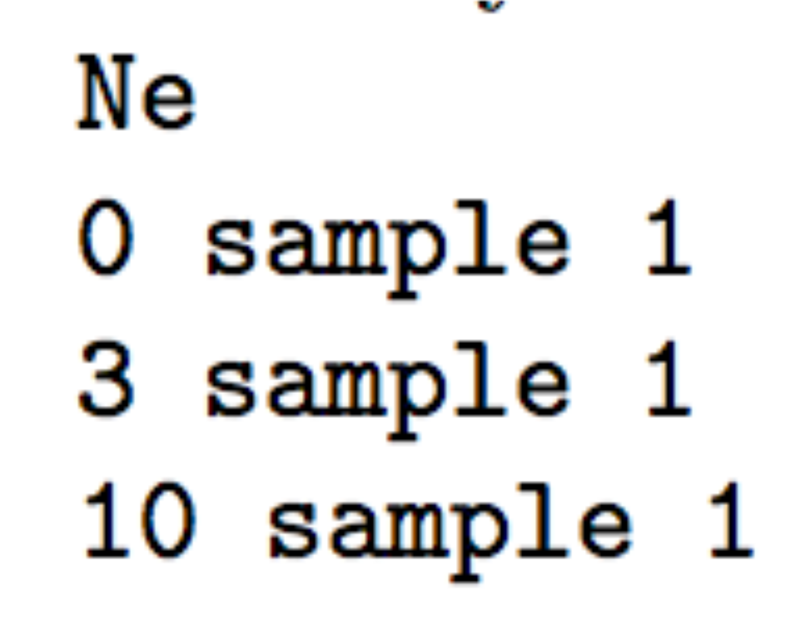
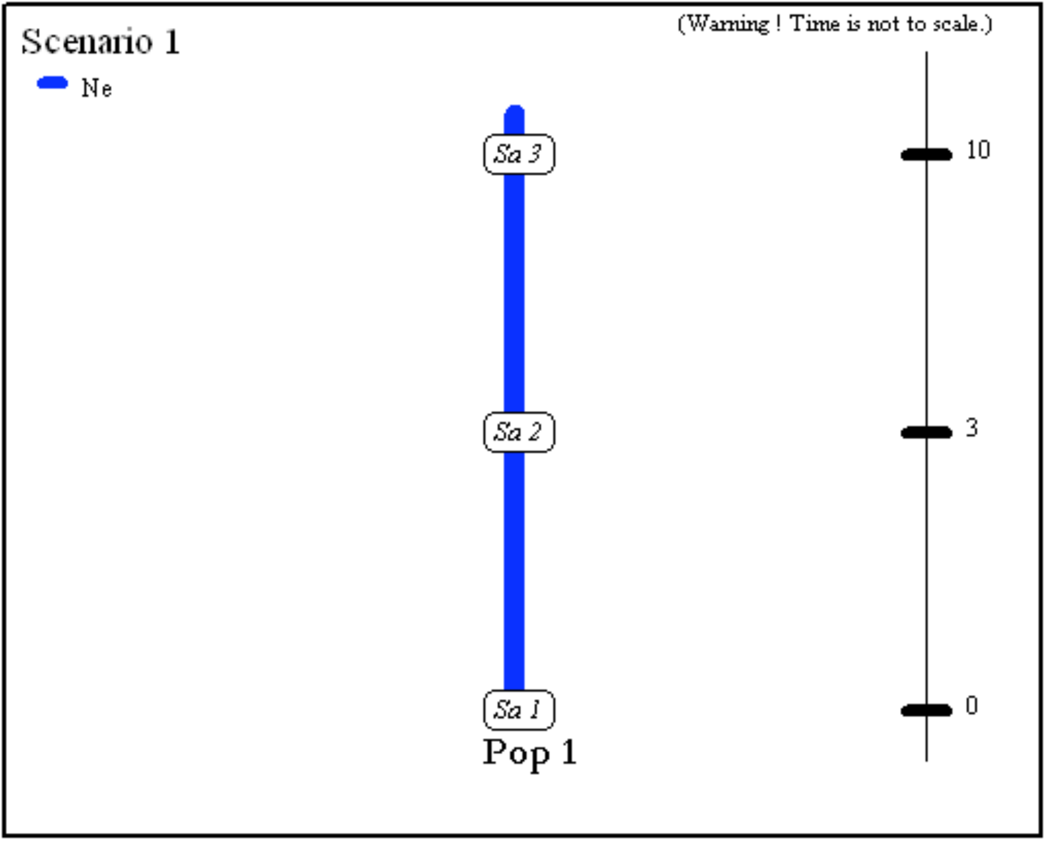
One population from which several samples have been taken at various generations: 0, 3 and 10. Generation 0 could correspond for instance to the most recent sampling date. The only unknown historical-demographical parameter of the scenario is the (constant) effective population size which is defined in the first line at sampling time.

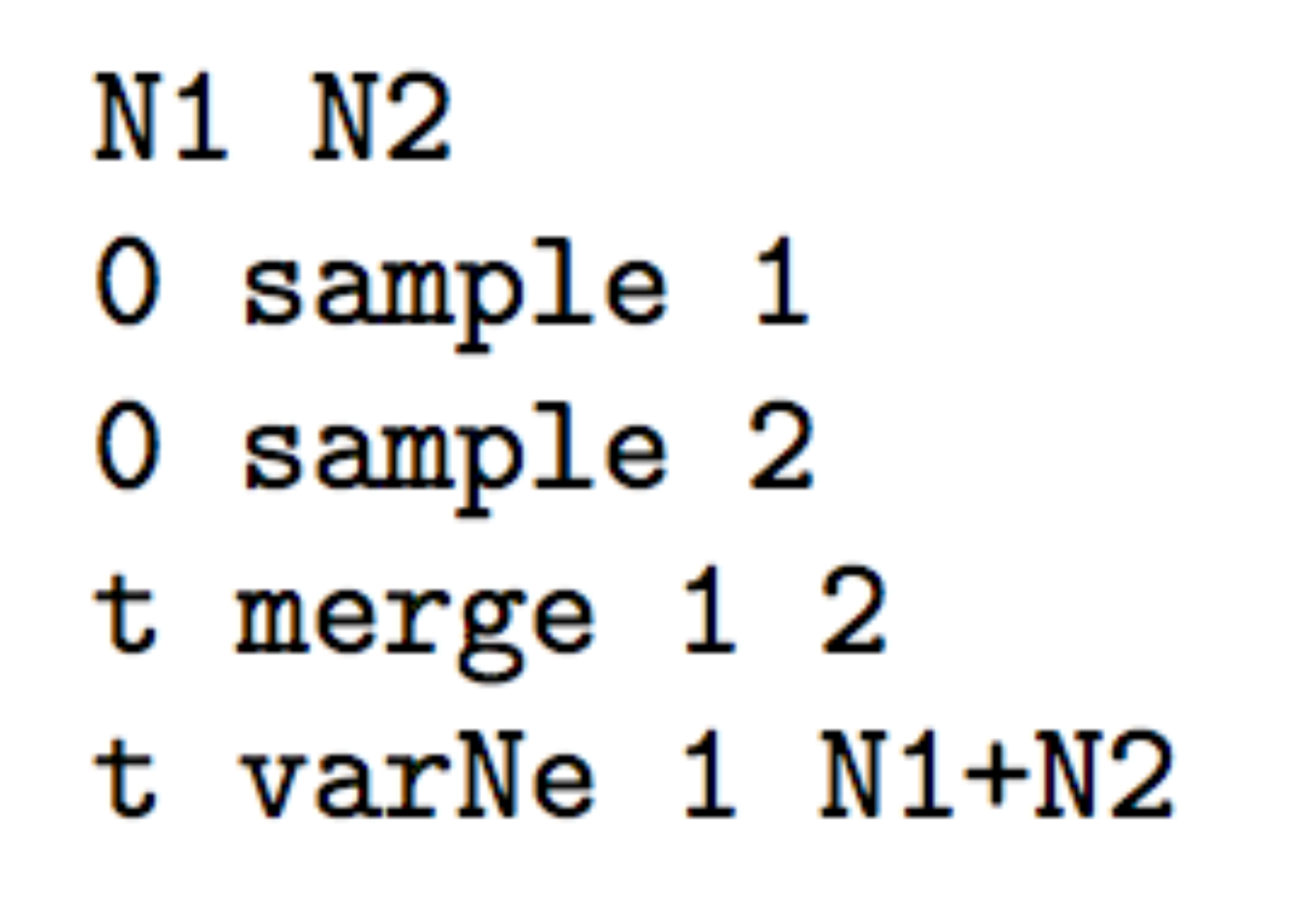
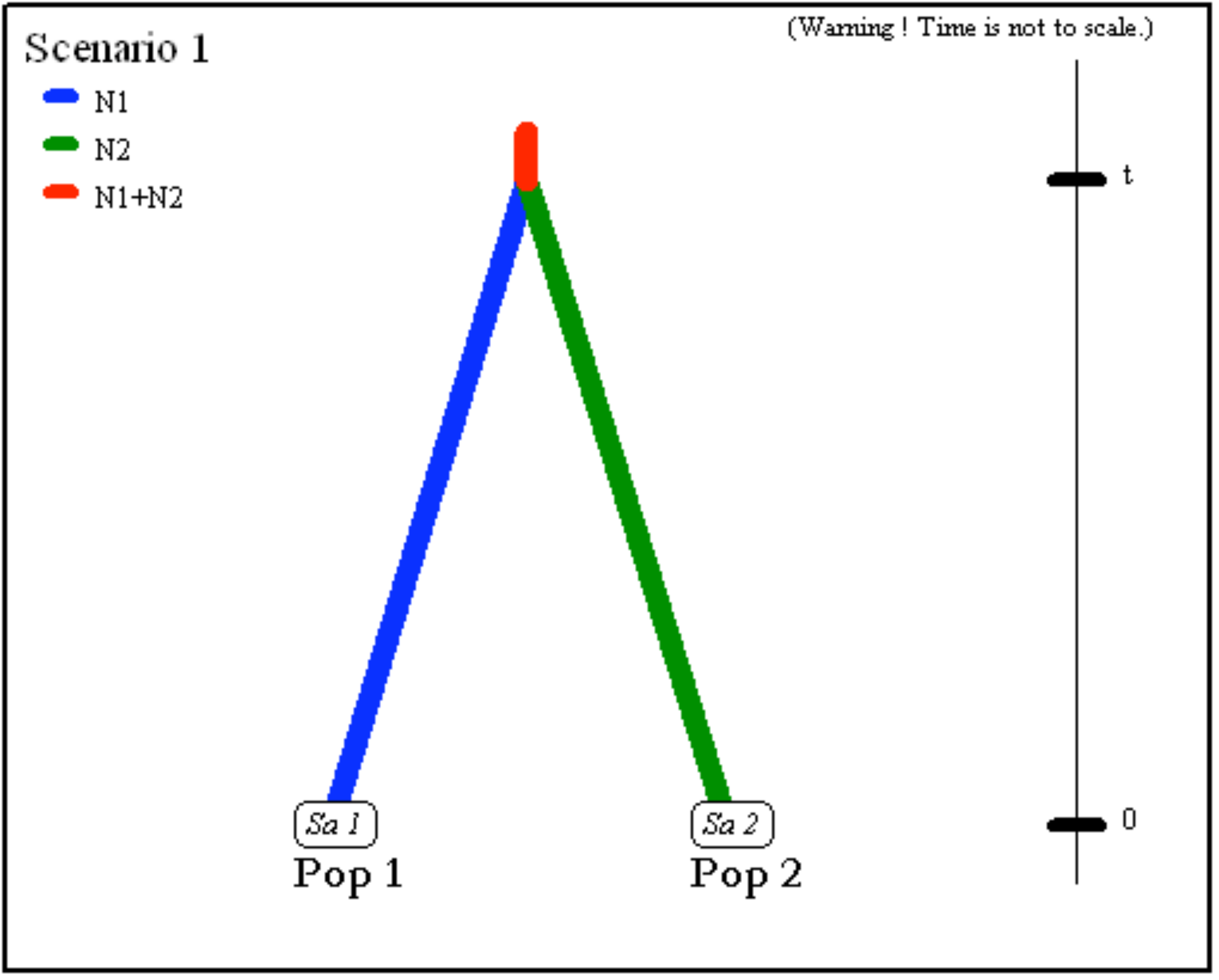
Two populations of size N1 and N2 (defined in the first line at sampling time) have diverged t generations in the past from an ancestral population of size N1+N2.

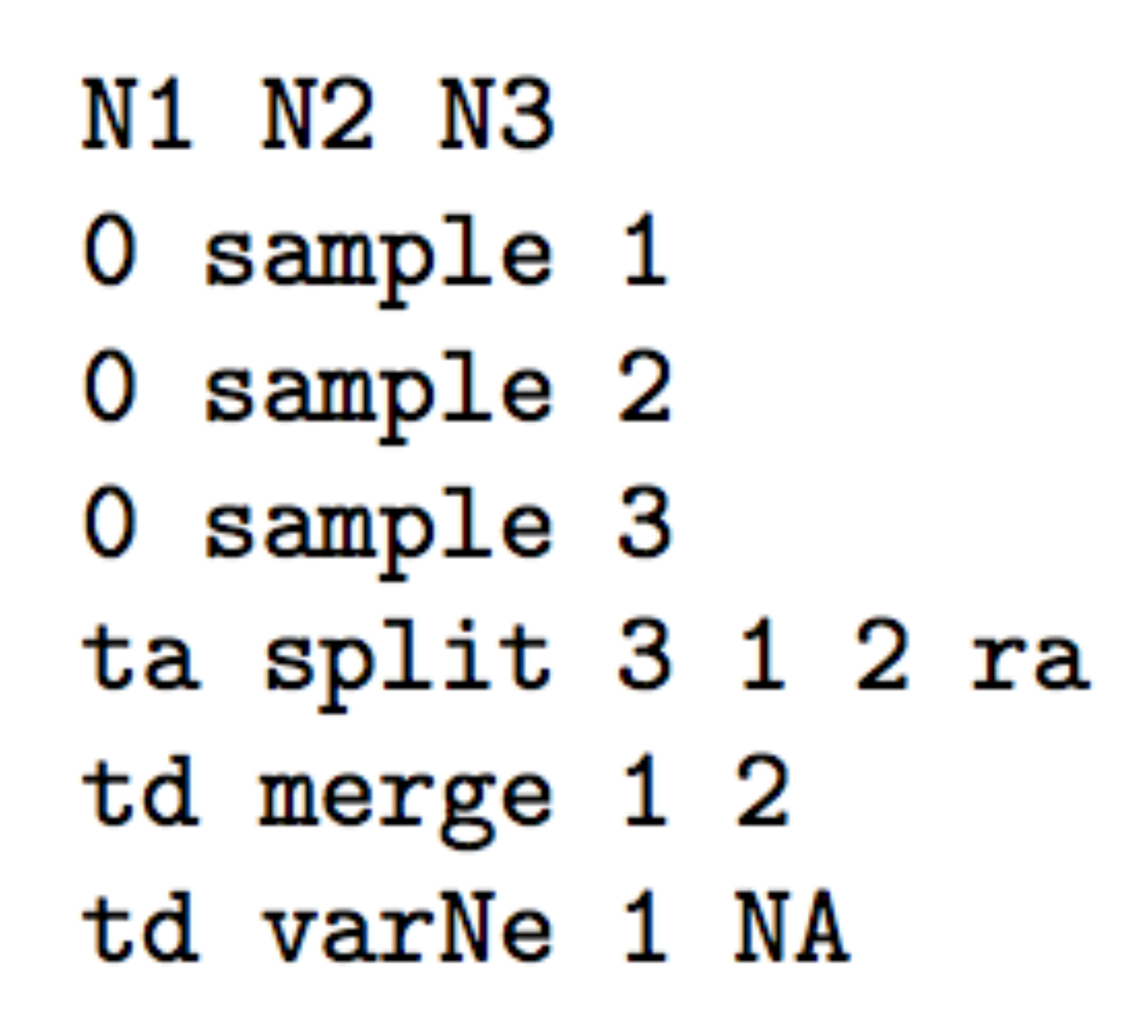
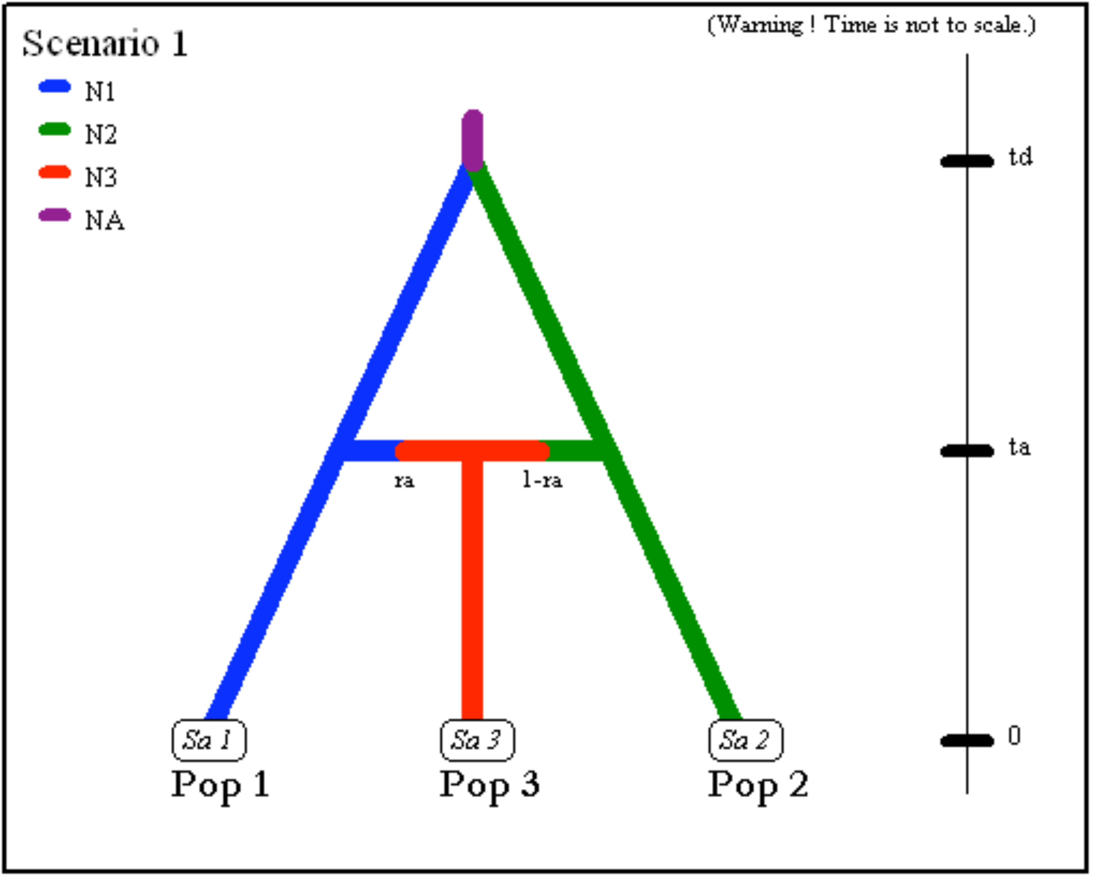
Two parental populations (1 and 2) with constant effective population sizes N1 and N2 have diverged at time td from an ancestral population of size NA. At time ta, there has been an admixture event between the two populations giving birth to an admixed population (3) with effective size N3 and with an admixture rate ra corresponding to the proportion of genes from population 1.

The next scenario includes four population samples and two admixture events. All populations have identical effective sizes (Ne).

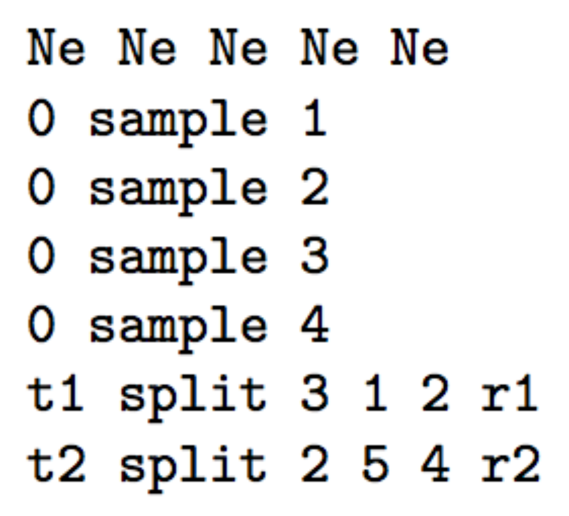
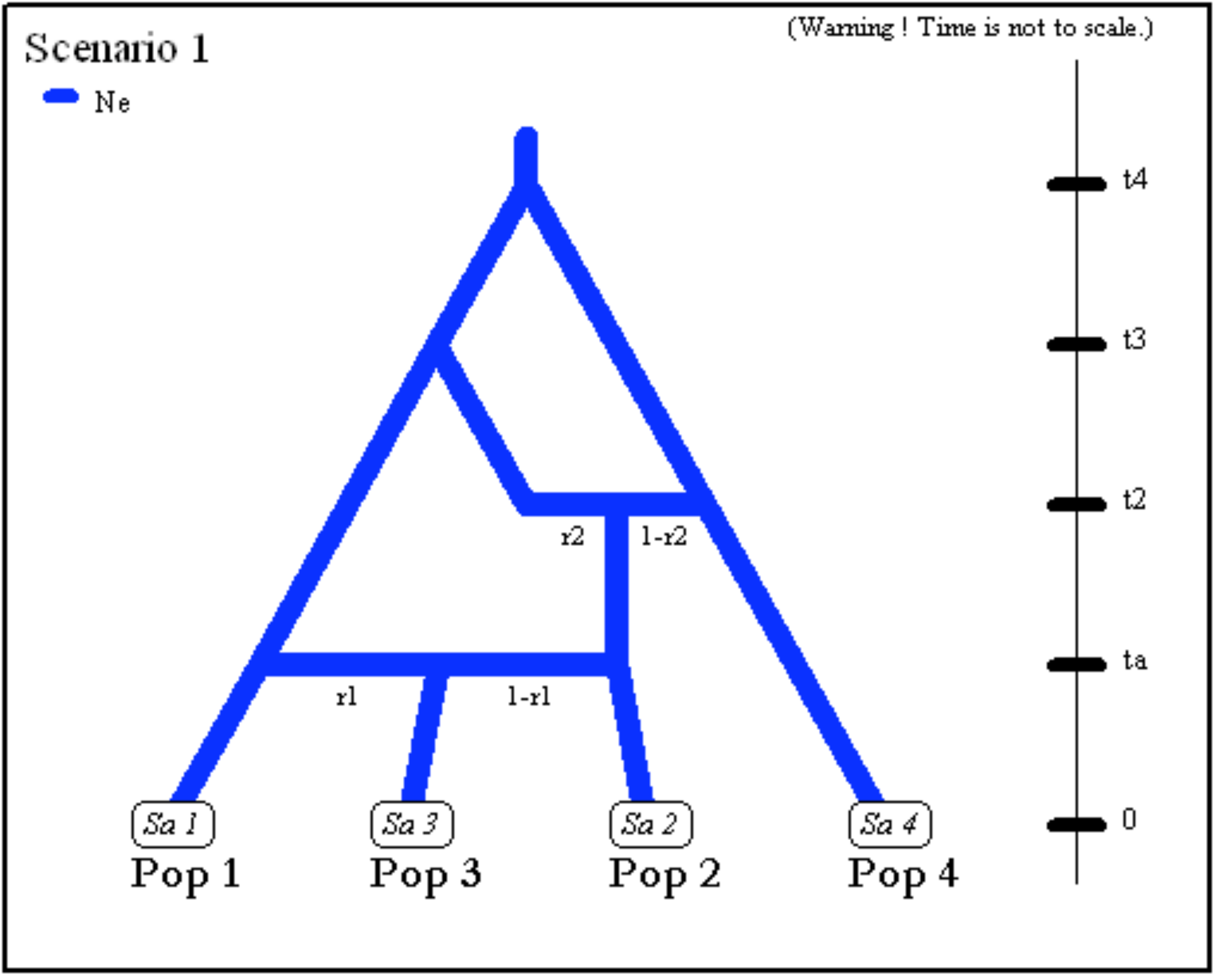
Note that although there are only four samples, the scenario includes a fifth unsampled population (also called “ghost population”). This unsampled population which diverged from population 1 at time t3 was a parent in the admixture event occurring at time t2. Note also that the first line must include the effective sizes (here Ne) of the five populations. (i.e. the four sampled population and the single unsampled population here at position 5).

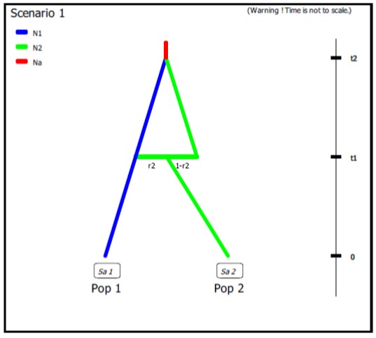
Example of DIYABC-RF code for unidirectional admixture/introgression where a fraction r2 of genes from population ‘Pop 2’ (with an effective population size N2) introgresses into population ‘Pop 1’ (with a population size N1) at time t1. The code also describes the merge of the two populations ‘Pop 1’ and ‘Pop 2’ into a common ancestor (with a population size Na) at time t2. It is worth noting that: (i) in the observed datafile, there are only two sampled populations (Pop 1 and Pop 2) and the user will need to define two (additional) unsampled populations in the first line of code (Pop 3 and Pop 4 with effective population size N2); (ii) we advise in this case to draw the fraction of genes transferred during the unidirectional admixture (r2) into a uniform distribution with min and max bounds equal to e.g.. 0.01 (very weak introgression from ‘Pop 2’ into ‘Pop 1’) and 0.5 (strong introgression from ‘Pop 2’ into ‘Pop 1’), respectively.

N1 N2 N2 N2 # comment 1

0 sample 1

0 sample 2

t1 split 2 3 4 r2 # comment 2

t1 merge 1 3 # comment 3

t2 merge 1 4 # comment 4

t2 VarNe 1 Na # comment 5

# comment 1: both unsampled populations ‘Pop 3’ and ‘Pop 4’ correspond to ‘Pop 2’, hence their population sizes N2.
# comment 2: at time t1 a fraction r2 of genes from ‘Pop 2’ goes into the unsampled population ‘Pop 3’ and a fraction 1-r2 goes into the unsampled population ‘Pop 4’ (‘Pop 2’ disappears)

# comment 3: we immediately merge (cf. still at time t1) the unsampled population ‘Pop 3’ (with the fraction r2 of genes from ‘Pop 2’) into the population ‘Pop 1’ - hence the unidirectional admixture of r2 genes from ‘Pop 2’ into ‘Pop 1’ (‘Pop 3’ disappears)

# comment 4: ‘Pop 4’ which now corresponds to the ex-‘Pop 2’ with the fraction 1-r2 of genes - can be merge into ‘Pop 1’

# comment 5: the population ancestral to ‘Pop 1’ and ‘Pop 2’ now has its own population size Na

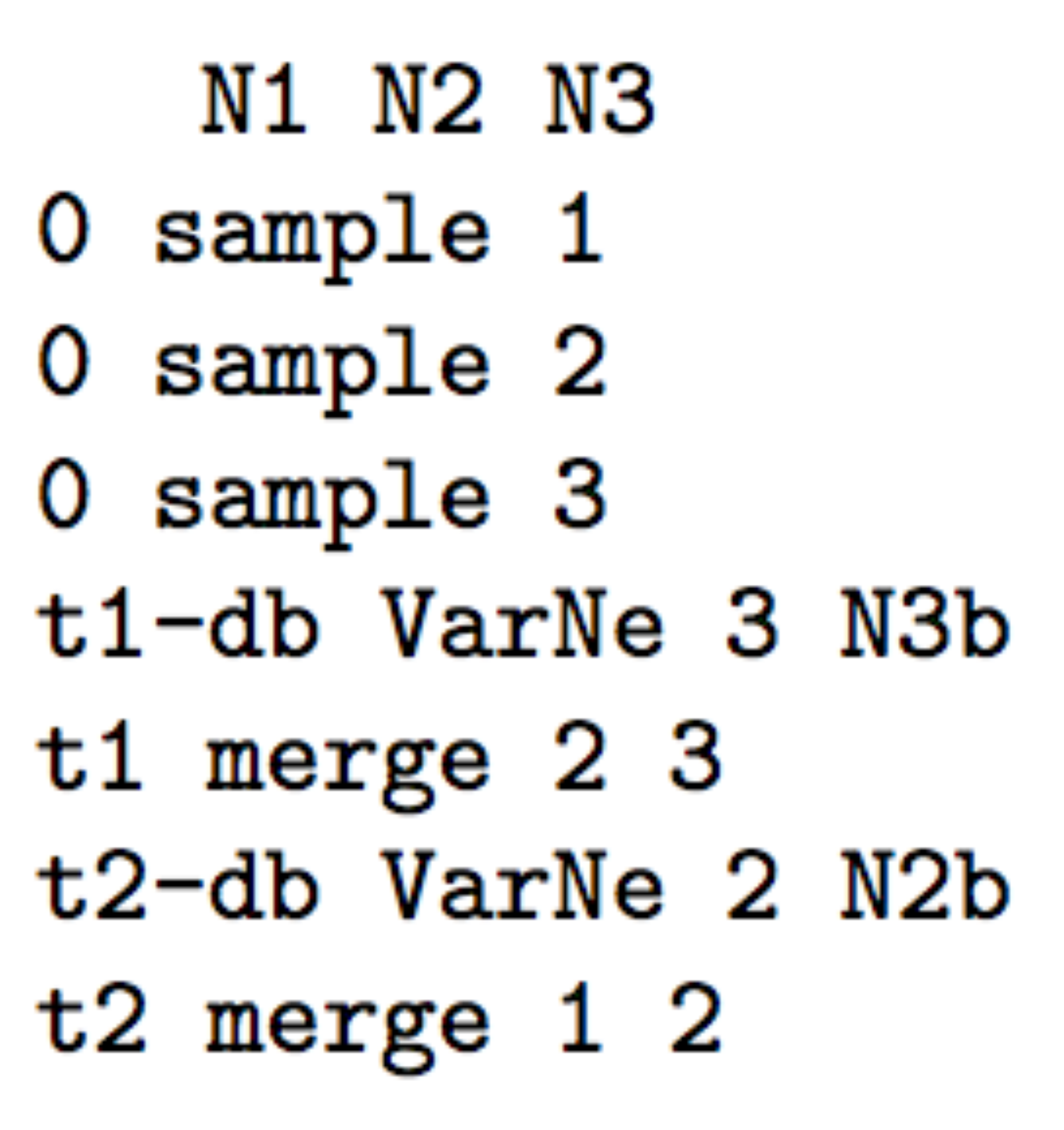
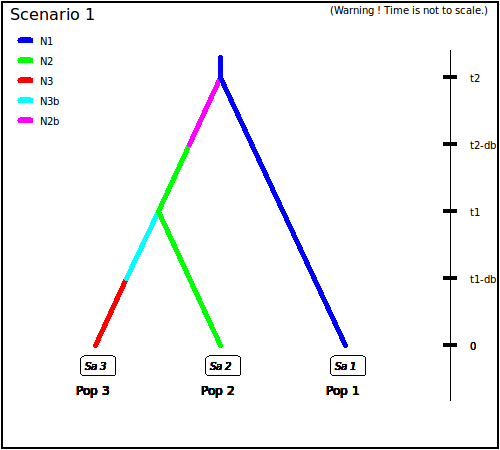
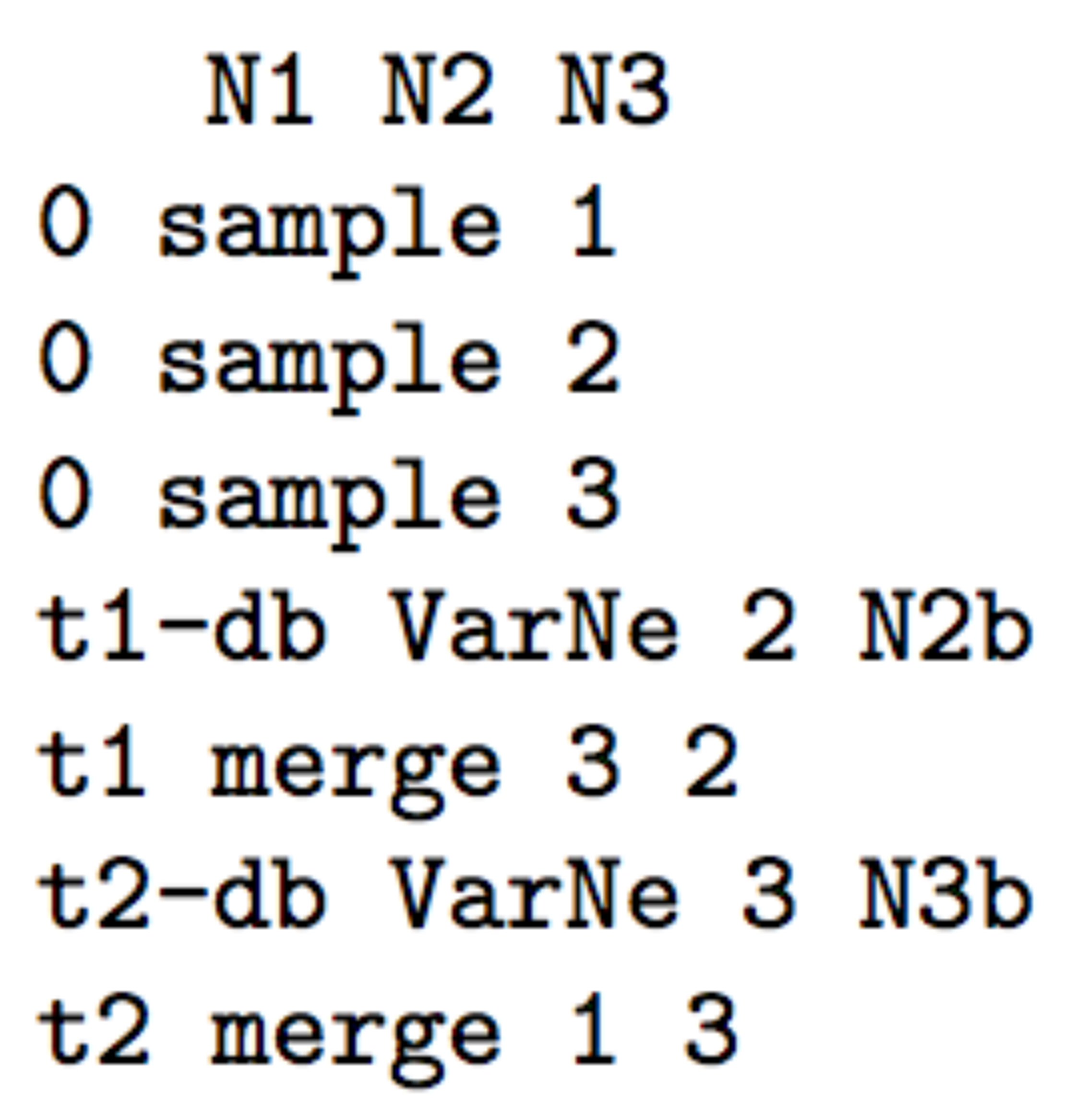
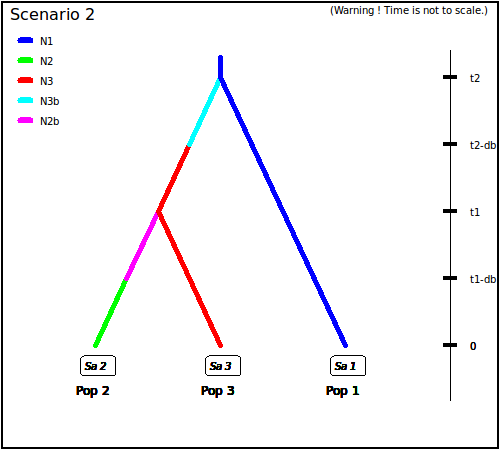
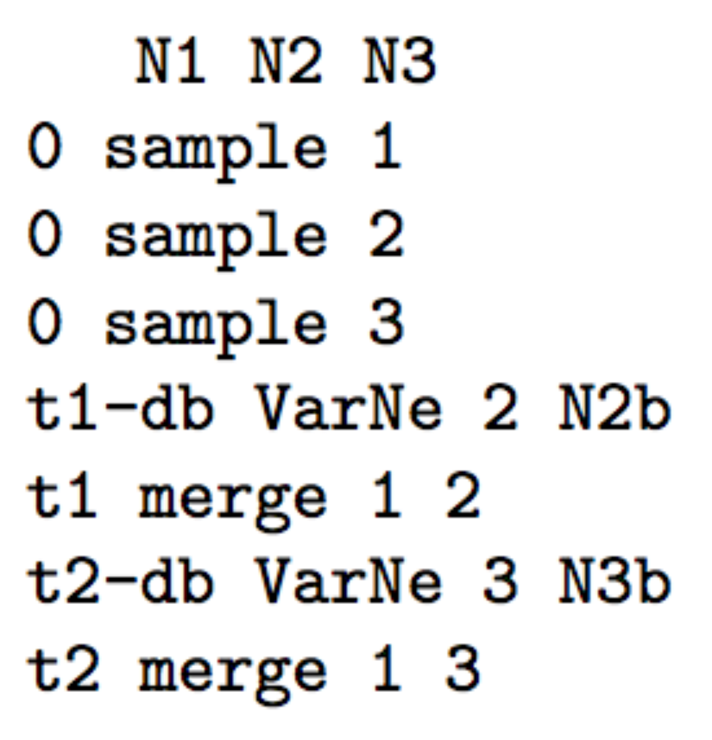
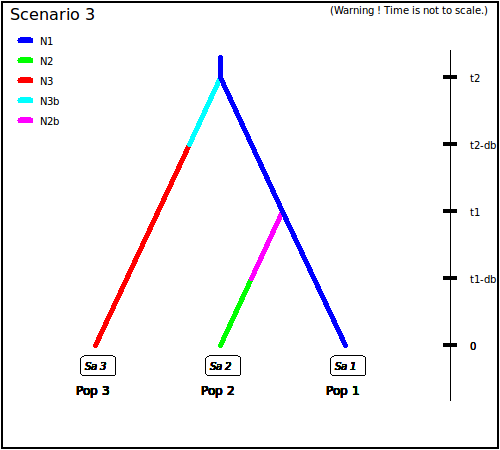
The following three scenarios correspond to a classic invasion history from an ancestral population (population 1). In scenario 1, population 3 is derived from population 2, itself derived from population 1. In scenario 2, population 2 derived from population 3, itself derived from population 1. In scenario 3, both populations 2 and 3 derived independently from population 1. Note that when a new population is created from its ancestral population, there is an initial size reduction (noted here N2b for population 2 and N3b for population 3) for a given number of generation (here db for both populations) mimicking a demographic bottleneck since the invasive population generally starts with a few immigrants. For instance, a low number of Nxb individuals for db generations could corresponds to Nxb values ranging between 5 to 100 individuals and db values ranging from 1 to 10 generations (e.g. Fraimout et al. 2017). If db = 0 then no bottleneck occurs which can be also a coding choice.

Scenario 1

Scenario 2

Scenario 3

2.4 Mutation model parameterization (microsatellite and DNA sequence loci)

The program can analyze microsatellite data and DNA sequence data altogether as well as separately. SNP loci can only be also analyzed separately from microsatellite data and DNA sequence data. It is worth stressing that all loci in an analysis must be genetically independent. Second, for DNA sequence loci, intra-locus recombination is not considered. Loci are grouped by the user according to its needs. For microsatellite and DNA sequence, a different mutation model can be defined for each group. For instance, one group can include all microsatellites with motifs that are 2 bp long and another group those with a 4 bp long motif. Also, with DNA sequence loci, nuclear loci can be grouped together and a mitochondrial locus form a separate group. SNPs do not require mutation model parameterization (see below for details).

We now describe the parameterization of microsatellite and DNA sequence markers.

2.4.1 Microsatellite loci

Although a variety of mutation models have been proposed for microsatellite loci, it is usually sufficient to consider only the simplest models (e.g. Estoup et al. 2002). This has the non-negligible advantage of reducing the number of parameters. This is why we chose the Generalized Stepwise Mutation model (GSM). Under this model, a mutation increases or decreases the length of the microsatellite by a number of repeated motifs following a geometric distribution. This model necessitates only two parameters: the mutation rate (µ) and the parameter of the geometric distribution (P). The same mutation model is imposed to all loci of a given group. However, each locus has its own parameters (µ_i and P_i) and, following a hierarchical scheme, each locus parameter is drawn from a gamma distribution with mean equal to the mean parameter value.

Note also that:

Individual loci parameters (µi and Pi) are considered as nuisance parameters and hence are never recorded. Only mean parameters are recorded.
The variance or shape parameter of the gamma distributions are set by the user and are NOT considered as parameters.
The SMM or Stepwise Mutation Model is a special case of the GSM in which the number of repeats involved in a mutation is always one. Such a model can be easily achieved by setting the maximum value of mean P ($\overline{P}$) to 0. In this case, all loci have their $P_{i}$ set equal to 0 whatever the shape of the gamma distribution.
All loci can be given the same value of a parameter by setting the shape of the corresponding gamma distribution to 0 (this is NOT a limiting case of the gamma, but only a way of telling the program).

To give more flexibility to the mutation model, the program offers the possibility to consider mutations that insert or delete a single nucleotide to the microsatellite sequence by using a mean parameter (named $\mu_{(SNI)}$) with a prior to be defined and individual loci having either values identical to the mean parameter or drawn from a Gamma distribution.

2.4.2 DNA sequence loci

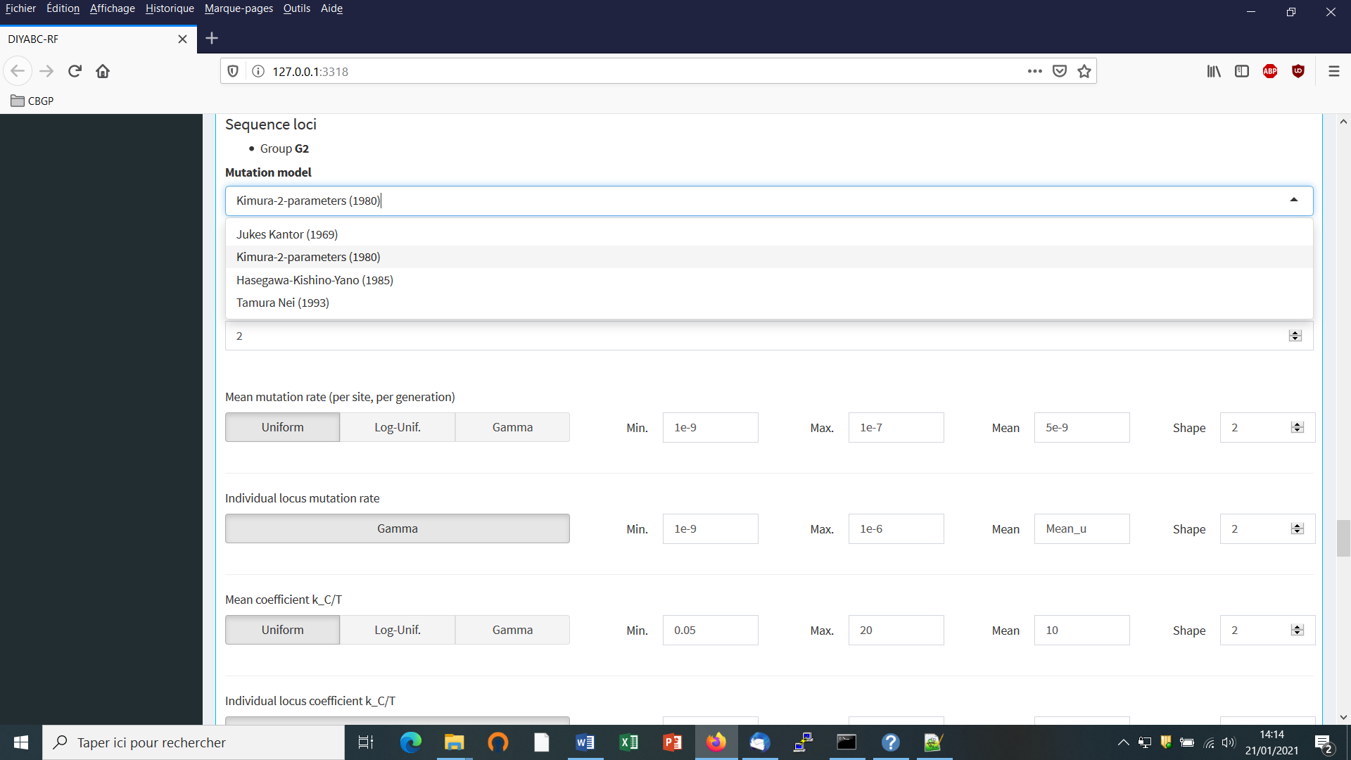
The program does not consider insertion-deletion mutations, mainly because there does not seem to be much consensus on this topic. Concerning substitutions, only the simplest models are considered. We chose the Jukes-Cantor (1969) one parameter model, the Kimura (1980) two parameter model, the Hasegawa-Kishino-Yano (1985) and the Tamura-Nei (1993) models. The last two models include the ratios of each nucleotide as parameters. In order to reduce the number of parameters, these ratios have been fixed to the values calculated from the observed dataset for each DNA sequence locus. Consequently, this leaves two and three parameters for the Hasegawa-Kishino-Yano (HKY) and Tamura-Nei (TN), respectively. Also, two adjustments are possible: one can fix the fraction of constant sites (those that cannot mutate) on the one hand and the shape of the Gamma distribution of mutations among sites on the other hand. As for microsatellites, all sequence loci of the same group are given the same mutation model with mean parameter(s) drawn from priors and each locus has its own parameter(s) drawn from a Gamma distribution (same hierarchical scheme). Notes 1, 2 and 4 of previous subsection (2.4.1) apply also for sequence loci.

2.4.3 SNPs do not require mutation model parameterization – notion of MAF and MRC

SNPs have two characteristics that allow to get rid of mutation models: they are (necessarily) polymorphic and they present only two allelic states (ancestral and derived). In order to be sure that all analyzed SNP loci have the two characteristics, monomorphic loci are discarded right from the beginning of analyses (when the observed dataset is scanned by the program). Note that a warning message will appear if the observed dataset include monomorphic loci, the latter being automatically removed from further analyses by the program. It is assumed that there occurred one and only one mutation in the coalescence tree of sampled genes. We will see below that this largely simplifies (and speeds up) SNP data simulation as one can use in this case the efficient “-s” algorithm of Hudson (2002) (Cornuet et al. 2014). Also, this advantageously reduces the dimension of the parameter space as mutation parameters are not needed in this case. There is however a potential drawback which is the absence of any calibration generally brought by priors on mutation parameters. Consequently, time/effective size ratios rather than original time or effective size parameters can be accurately estimated (e.g. Collin et al. 2021).

It is worth noting that, using the Hudson’s simulation algorithm for SNP markers leads to applying a kind of default MAF (minimum allele frequency) criterion on the simulated dataset. As a matter of fact, with this simulation algorithm each locus in both the observed and simulated datasets will be characterized by the presence of at least one copy of the SNP alleles over all genes sampled from all studied populations (i.e. pooling all genes genotyped at the locus). In DIYABC-RF, it is possible to impose a different MAF criterion on both the observed and simulated datasets. For each SNP, the MAF is computed pooling all genes genotyped over all studied population samples. For instance, the specification of a MAF equal to 5% will automatically select a subset of m loci characterized by a minimum allele frequency ≥ 5% out of the l loci of the observed dataset and only m loci with a MAF ≥ 5% will be retained in a simulated dataset. In practice, the instruction for a given MAF has to be indicated directly in the headline of the file of the observed dataset (see section 7.1.1 for data file examples). For instance, if one wants to consider only loci with a MAF equal to 5% one will write <MAF=0.05> in the headline. Writing <MAF=hudson> (or omitting to write any instruction with respect to the MAF) will bring the program to use the standard Hudson’s algorithm without further selection. The selection of a subset of loci fitting a given MAF allows: (i) to remove loci with very low level of polymorphism from the dataset and hence increase the mean level of genetic variation of both the observed and simulated datasets, without producing any bias in the analyses; and (ii) to reduce the proportion of loci for which the observed variation may corresponds to sequencing errors. In practice MAF values ≤10% are considered. To check for the consistency/robustness of the ABC results obtained, it may be useful to treat a SNP dataset considering different MAFs (for instance MAF=hudson, MAF=1% and MAF=5%). Note that increasing the MAF leads to increase the simulation times of SNP datasets as more loci need to be simulated with the Hudson’s algorithm to obtain a given number of loci fitting the required MAF.

It is worth stressing that the MAF criterion applies to standard Individual sequencing (hereafter IndSeq) SNP data. In addition to IndSeq data, DIYABC-RF allows the simulation and analyses of pool-sequencing SNP data (hereafter PoolSeq data), which basically consist of whole-genome sequences of pools of tens to hundreds of individual DNAs (Gautier et al. 2013; Schlötterer et al. 2014). In practice, the simulation of PoolSeq data consists first in simulating individual SNP genotypes for all individuals in each population pool, and then generating pool read counts from a binomial distribution parameterized with the simulated allele counts (obtained from individual SNP genotypes) and the total pool read coverage (e.g., Hivert et al. 2018). A criterion somewhat similar to the MAF was implemented for PoolSeq data: the minimum read count (MRC). The MRC is the minimum number of sequence reads for each alleles of a SNP when pooling the reads overall population samples. The specification of a MRC equal for instance to 5 will automatically select a subset of m PoolSeq loci for which both alleles have at least five reads among the l loci of the observed dataset and only m loci with a MRC ≥ 5 will be retained in a simulated dataset. In practice, the instruction for a given MRC has to be indicated directly in the headline of the file of the observed dataset (see section 7.1.2 for data file examples). For instance, if one wants to consider only loci with a MRC equal to 5 one will write <MRC=5> in the headline. The selection of a subset of loci fitting a given MRC allows to reduce the proportion of loci for which the observed variation may corresponds to sequencing errors. If MRC is large enough (e.g. MRC=5 or 10), it also removes the loci with very low level of polymorphism from the dataset and hence increase the mean level of genetic variation of both the observed and simulated datasets, without producing any bias in the analyses; In practice MRC values of 2, 3,4 and 5 are recommended. To check for the consistency/robustness of the ABC results obtained, it may be useful to treat a SNP dataset considering different MAFs (for instance MRC=2 and MRC=5). As for the MAF, increasing the MRC leads to increase the simulation times of PoolSeq SNP datasets as more loci need to be simulated with the Hudson’s algorithm to obtain a given number of loci fitting the required MRC.

2.5 Prior distributions

The Bayesian aspect of the ABC-RF approach implies that parameter estimations use prior knowledge about these parameters that is given by prior distributions of parameters. The program offers a choice among usual probability distributions, i.e. Uniform, Log-Uniform, Normal or Log-Normal for historical parameters and Uniform, Log-Uniform or Gamma for mutation parameters. Extremum values (min and max) and other parameters (e. g. mean and standard deviation) must be filled in by the user. It is worth noting that one can impose some simple conditions on historical parameters. For instance, there can be two times parameters with overlapping prior distributions. However, we want that the first one, say t1, to always be larger than the second one, say t2. For that, we just need to set t1>t2 in the corresponding edit-windows. Such a condition needs to be between two parameters and more precisely between two parameters of the same category (i.e. two effective sizes, two times or two admixture rates). The limit to the number of conditions is imposed by the logics, not by the program. The only binary relationships accepted here are <, >, ≤, and ≥.

2.6 Summary statistics as components of the feature vector

The training set includes values of a feature vector which is a multidimensional representation of any data point (i.e. simulated or observed datasets) made up of measurements (or features) taken from it. More specifically, the feature vector includes a large number of statistics that summarize genetic variation in the way that they allow capturing different aspects of gene genealogies and hence various features of molecular patterns generated by selectively neutral population histories (e.g. Beaumont 2010; Cornuet et al. 2014). For each category (microsatellite, DNA sequences or SNP) of loci, the program proposes a series of summary statistics among those used by population geneticists.

Note: The code name of each statistic mentioned in the various program outputs is given between brackets [XXX] in sections 2.6.1, 2.6.2 and 2.6.3.

2.6.1 For microsatellite loci

Single sample statistics:

[NAL] - mean number of alleles across loci
[HET] - mean gene diversity across loci (Nei 1987)
[VAR] - mean allele size variance across loci
[MGW] - mean M index across loci (Garza and Williamson 2001; Excoffier et al. 2005)

Two sample statistics:

[N2P] - mean number of alleles across loci (two samples)
[H2P] - mean gene diversity across loci (two samples)
[V2P] - mean allele size variance across loci (two samples)
[FST] -$F_{ST}$ between two samples (Weir and Cockerham 1984)
[LIK] - mean index of classification (two samples)

(Rannala and Moutain 1997; Pascual et al. 2007)

[DAS] - shared allele distance between two samples (Chakraborty and Jin 1993)
[DM2] - distance between two samples (Golstein et al. 1995)

Three sample statistics:

[AML] - Maximum likelihood coefficient of admixture (Choisy et al. 2004)

2.6.2 For DNA sequence loci

Single sample statistics:

[NHA] - number of distinct haplotypes
[NSS] - number of segregating sites
[MPD] - mean pairwise difference
[VPD] - variance of the number of pairwise differences
[DTA] - Tajima’s D statistics (Tajima 1989)
[PSS] - Number of private segregating sites

(=number of segregating sites if there is only one sample)

[MNS] - Mean of the numbers of the rarest nucleotide at segregating sites
[VNS] - Variance of the numbers of the rarest nucleotide at segregating sites

Two sample statistics:

[NH2] - number of distinct haplotypes in the pooled sample
[NS2] - number of segregating sites in the pooled sample
[MP2] - mean of within sample pairwise differences
[MPB] - mean of between sample pairwise differences
[HST] -$F_{ST}$ between two samples (Hudson et al. 1992)

Three sample statistics:

[SML] Maximum likelihood coefficient of admixture (adapted from Choisy et al. 2004)

2.6.3 For SNP loci

For both IndSeq and PoolSeq SNPs, we have implemented the following (same) set of summary statistics.

1. [ML1p] [ML2p] [ML3p] [ML4p] - Proportion of monomorphic loci for each population, as well as for each pair, triplet and quadruplet of populations.

Mean (m suffix added to the code name) and variance (v suffix) over loci values are computed for all subsequent summary statistics

2. [HWm] [HWv] [HBm] [HBv] - Heterozygosity for each population and for each pair of populations (Hivert et al. 2018).

3. [FST1m] [FST1v] [FST2m] [FST2v] [FST3m] [FST3v] [FST4m] [FST4v] [FSTGm] [FSTGv] - FST-related statistics for each population (i.e., population-specific FST; Weir & Goudet 2017), for each pair, triplet, quadruplet and overall populations (when the dataset includes more than four populations) (Hivert et al. 2018).

4. [F3m] [F3v] [F4m] [F4v] – allele shared Patterson’s f-statistics for each triplet (f3-statistics) and quadruplet (f4-statistics) of populations (Patterson et al. 2012 and Leblois et al. 2018 for the PoolSeq unbiased f3-statistics)

5. [NEIm] [NEIv] - Nei’s (1972) distance for each pair of populations

6. [AMLm] [AMLv] - Maximum likelihood coefficient of admixture computed for each triplet of populations (adapted from Choisy et al. 2004).

2.7 Generating the training set

The training set can include as many scenarios as desired. The prior probability of each scenario is uniform so that each scenario will have approximately the same number of simulated datasets. Only parameters that are defined for the drawn scenario are generated from their respective prior distribution. Scenarios may or may not share parameters. When conditions apply to some parameters (see section 2.3), parameter sets are drawn in their respective prior distributions until all conditions are fulfilled. The simulated datasets (summarized with the statistics detailed in section 2.6) of the training set are recorded for further statistical analyses (using Random Forest algorithms) in a key binary file named reftableRF.bin.

3. RANDOM FOREST ANALYSIS

Once the training set has been generated, one can start various statistical treatments using the Random Forest (RF) algorithms implemented in the program and by running the “Random Forest analyses” module.

3.1 Addition of linear combinations of summary statistics to the vector feature

For scenario choice, the feature vector can be enriched before processing RF predictions (default option that can be disabled) by values of the d axes of a linear discriminant analysis (LDA) processed on the above summary statistics (with d equal to the number of scenarios minus 1; Pudlo et al. 2016). In the same spirit, for parameter estimation, the feature vector can be completed (default option that can be disabled) by values of a subset of the s axes of a Partial Least Squares Regression analysis (PLS) also processed on the above summary statistics (with s equal to the number of summary statistics). The number of PLS axes added to the feature vector is determined as the number of PLS axes providing a given fraction of the maximum amount of variance explained by all PLS axes (i.e., 95% by default, but this parameter can be adjusted). Note that, according to our own experience on this issue, the addition into the feature vector of LDA or PLS axes better extract genetic information from the training set and hence globally improved statistical inferences. While the inferential gain turned out to be systematic and substantial for LDA axes (scenario choice), we found that including PLS axes improved parameter estimation in a heterogeneous way, with a negligible gain in some cases (e.g. Collin et al. 2020).

3.2 Prediction using Random Forest: scenario choice

For scenario choice, the outcome of the first step of RF prediction applied to a given target dataset is a classification vote for each scenario which represents the number of times a scenario is selected in a forest of n trees. The scenario with the highest classification vote corresponds to the scenario best suited to the target dataset among the set of compared scenarios. This first RF predictor is good enough to select the most likely scenario but not to derive directly the associated posterior probabilities. A second analytical step based on a second Random Forest in regression is necessary to provide an estimation of the posterior probability of the best supported scenario (Pudlo et al. 2016).

3.3 Prediction using Random Forest: parameter estimation

For parameter estimation, Raynal et al. (2019) extended the RF approach developed in the context of (non-parametric) regression to estimate the posterior distributions of a given parameter under a given scenario. The approach requires the derivation of a new Random Forest for each component of interest of the parameter vector (i.e. “one parameter, one forest strategy”; Raynal et al. 2019). Quite often, practitioners of Bayesian inference report the posterior mean, posterior variance or posterior quantiles, rather than the full posterior distribution, since the former are easier to interpret than the latter. We implemented in DIYABC-RF the methodologies detailed in Raynal et al. (2019) to provide estimations of the posterior mean, variance, median (i.e. 50% quantile) as well as 5% and 95% quantiles (and hence 90% credibility interval) of each parameter of interest. The posterior distribution of each parameter of interest is also inferred using importance weights following Meinshausen (2006)’s work on quantile regression forests.

3.4 Assessing the quality of predictions

To evaluate the robustness of inferences, DIYABC-RFt provides:

Global (i.e. prior) error/accuracy metrics corresponding to prediction quality measures computed over the entire data space;
Local (i.e. posterior) error/accuracy metrics computed conditionally on the observed dataset and hence corresponding to prediction quality exactly at the position of the observed dataset.

Note that the program used the out-of-bag prediction method for estimating global and local error/accuracy measures (Pudlo et al. 2016; Raynal et al. 2019; Chapuis et al. 2020). The out-of-bag dataset corresponds to the data of the training set that were not selected when creating the different tree bootstrap samples and is hence equivalent to using an independent test dataset (Breiman, 2001; Pudlo et al. 2016; Raynal et al. 2019). Using the out-of-bag prediction method for estimating global and local error/accuracy measures is computationally efficient as this approach makes use of the datasets already present in the training set and hence avoids the computationally costly simulations (especially for large SNP datasets) of additional test datasets.

3.4.1 Metrics for scenario choice

Global prior errors including the confusion matrix (i.e. the contingency table of the true and predicted classes – here scenarios - for each example in the training set) and the mean misclassification error rate (over all scenarios).
Local posterior error which corresponds to 1 minus the posterior probability of the selected scenario (Chapuis et al. 2020).

3.4.2 Metrics for parameter estimation

Global (prior) and local (posterior) NMAE (i.e. normalized mean absolute error): it is the average absolute difference between the point estimate and the true simulated value divided by the true simulated value, with the mean or the median taken as point estimate.
Global (prior) and local (posterior) MSE and NMSE (i.e. the mean square error): it is the average squared difference between the point estimate and the true simulated value for MSE, divided by the true simulated value for NMSE, again with the mean or the median taken as point estimate.
Several confidence interval measures computed only at the global (prior) scale:

- 90% coverage: it is the proportion of true simulated values located between the estimated 5% and 95% quantiles.

- Mean or median of the 90% amplitude: it is the mean or median of the difference between the estimated 5% and 95% quantiles.

- Mean or median of the relative 90% amplitude: it is the mean or median of the difference between the estimated 5% and 95% divided by the true simulated value.

4. PRACTICAL CONSIDERATIONS FOR ABC-RF TREATMENTS

Random Forest is often (positively) considered as a “tuning-free” method in the sense that it does not require meticulous calibrations. This represents an important advantage of this method (for instance compared to standard ABC methods, Neural Network methods and more sophisticated Deep Learning methods; Collin et al. 2020), especially for non-expert users. In practice, we nevertheless advise users to consider several checking points, thereafter formalized as questions, before finalizing inferential treatments using DIYABC-RF.

4.1 Are my scenarios and/or associated priors compatible with the observed dataset?

This question is of prime interest and applies to ABC-RF as well as to any alternative ABC treatments. This issue is particularly crucial, given that complex scenarios and high dimensional datasets (i.e., large and hence very informative datasets) are becoming the norm in population genomics. Basically, if none of the proposed scenario / prior combinations produces some simulated datasets in a reasonable vicinity of the observed dataset, this is a signal of incompatibility and it is not recommended to attempt any inferences. In such situations, we strongly advise reformulating the compared scenarios and/or the associated prior distributions in order to achieve some compatibility in the above sense. DIYABC-RF proposes a visual way to address this issue through the simultaneous projection of datasets of the training database and of the observed dataset on the first Linear Discriminant Analysis (LDA) axes. In the LDA projection, the (target) observed dataset has to be reasonably located within the clouds of simulated datasets. The program also proposes some complementary dedicated tools: (i) a Principal Component Analysis (PCA) representing on 2-axes plans the simulated dataset from the training set and the observed dataset; and (ii), for each summary statistics, the proportion of simulated data (considering the total training set) that have a value below the value of the observed dataset. A star indicates proportions lower than 5% or greater than 95% (two stars, <1% or >1%; three stars, <0.1% or >0.1%). The latter numerical results can help users to reformulating the compared scenarios and/or the associated prior distributions in order to achieve some compatibility (see e.g. Cornuet et al. 2010). See also the complementary and more basic procedure based on Principal Component Analysis (PCA) proposed in section “5.4.7 Step 7: Prior-scenario checking PRE-ANALYSIS (optional but recommended)”.

4.2 Did I simulate enough datasets for my training set?

A rule of thumb is, for scenario choice to simulate between 2,000 and 20,000 datasets per scenario among those compared (Pudlo et al. 2016; Estoup et al. 2018), and for parameter estimation to simulate between 10,000 and 100,000 datasets under a given scenario (Raynal et al. 2019; Chapuis et al. 2020). To evaluate whether or not this number is sufficient for RF analysis, we recommend to compute error/accuracy metrics such as those proposed by DIYABC-RF from both the entire training set and a subset of the latter (for instance from a subset of 80,000 simulated datasets if the training set includes a total of 100,000 simulated datasets). If error (accuracy) metrics from the subset are similar, or only slightly higher (lower) than the value obtained from the entire database, one can consider that the training set contains enough simulated datasets. If a substantial difference is observed between both values, then we recommend increasing the number of simulated datasets in the training set.

4.3 Did my forest frow enough trees?

According to our experience, a forest made of 500 to 2,000 trees often constitutes an interesting trade-off between computation efficiency and statistical precision (Breiman, 2001; Chapuis et al. 2020; Pudlo et al. 2016; Raynal et al. 2019). To evaluate whether or not this number is sufficient, we recommend plotting error/accuracy metrics as a function of the number of trees in the forest. The shapes of the curves provide a visual diagnostic of whether such key metrics stabilize when the number of trees tends to a given value. DIYABC-RF provides such a plot-figure as output.

5. RUNNING (EXAMPLE) DATASET TREATMENTS USING THE GRAPHIC USER INTERFACE (GUI)

5.1 Launching the GUI

The GUI is the standard and user-friendly interface to use the software DIYABC-RF. You can configure the required parameters and follow the progress directly in the interface and through log files. A given GUI session (i.e. a window) allows working on a single project. You can launch several GUI sessions (i.e. several windows) on a single computer hence allowing working on several projects in parallel.
When using the operating system Microsoft Windows, launch the GUI by double-clicking on the file DIYABC-RF_GUI.bat included in the DIYABC-RF_GUI_xxx_windows.zip file available from https://diyabc.github.io. When using MacOS, launch the GUI by double-clicking on the icon of the file DIYABC-RF_GUI.command included in the DIYABC-RF_GUI_xxx_macos.zip file available from https://diyabc.github.io

It is worth stressing that the program can also be run locally as any shiny application using R (only possibility on Linux). You can visit https://diyabc.github.io/gui/#r-package-installation for more details.

The main pipeline of DIYABC-RF includes two modules corresponding to the two main phases:

Module 1 = “Training set simulation” where users specify how simulated data will be generated under the ABC framework to produce a training set.

Module 2 = “Random Forest analysis” (necessitating the presence of a training set) which guides users through scenario choice and parameter inference by providing a simple interface for the supervised learning framework based on Random Forest methodologies.

An additional (auxiliary) module named “Synthetic data file generation” is also available from the GUI (cf. section 8). It can be used to easily generate data file(s) corresponding to synthetic “ground truth” raw data (not summarized through statistics) under a given historical scenario and a set of fixed parameter values, for instance for benchmarking purpose. The formats of such simulated data files are the same as those described in section 7.1 for observed (i.e. real) datasets for which one usually wants to make inferences.

5.2 What is a DIYABC-RF project?

A DIYABC-RF project consists of different files, related to the training set simulation and random forest analyses. A project includes at least one observed dataset and one header file associated to a (already generated or not) training set. The header file, named headerRF.txt, contains all information necessary to compute a training set associated with the data: i.e. the scenarios, the scenario parameter priors, the characteristics of loci, the loci parameter priors and the list of summary statistics to compute using the Training set simulation module. As soon as the first records of the training set have been simulated, they are saved in the training set file, named reftableRF.bin. In addition, the file statobsRF.txt, stores the value of the summary statistics computed from the observed dataset.

Outputs of Random forest analyses are available in sub-directories (each one corresponding to a specific setting that you may have configured for the random forest analyses) in the project directory; see the corresponding section 7.3 for more details regarding the content of outputs generated by a Random Forest analysis.

It is worth stressing that you need to SAVE a project to avoid losing your work before quitting the GUI. A project zip file will be generated and can be saved. If you want to later continue with a project, or clone/modify an existing project, you can provide the key files of an existing projec in the GUI when starting a project.

Finally, we strongly advised NOT to manually edit project-related files in a text editor, unless you know what you are doing!

5.3 Main options of the home screen

When launching the GUI, the home screen appears like this:

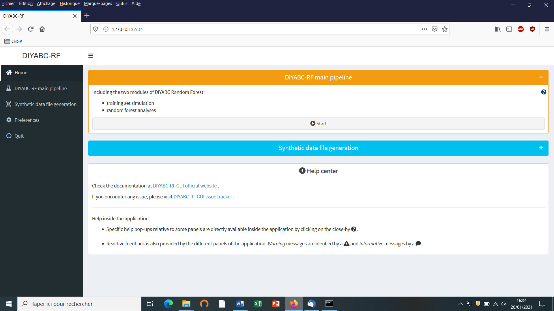
Access to main functionalities: you can access to the two main functionalities of the program (i.e. training set simulation and random forest analyses) in two ways: (i) by clicking on the “Start” button in the middle of the Home panel or (ii) by clicking on the “DIYABC-RF main pipeline” button in the upper-left part of the panel.
Access to other functionalities:

To access to the panels allowing generating files corresponding to full in silico datasets (also called pseudo-observed datasets) click on the “Synthetic data file generation” button in the middle of the panel or on the “Synthetic data file generation” button in the upper-left part of the panel.
Clicking on the “Preference” button (upper left) gives access to the following screen

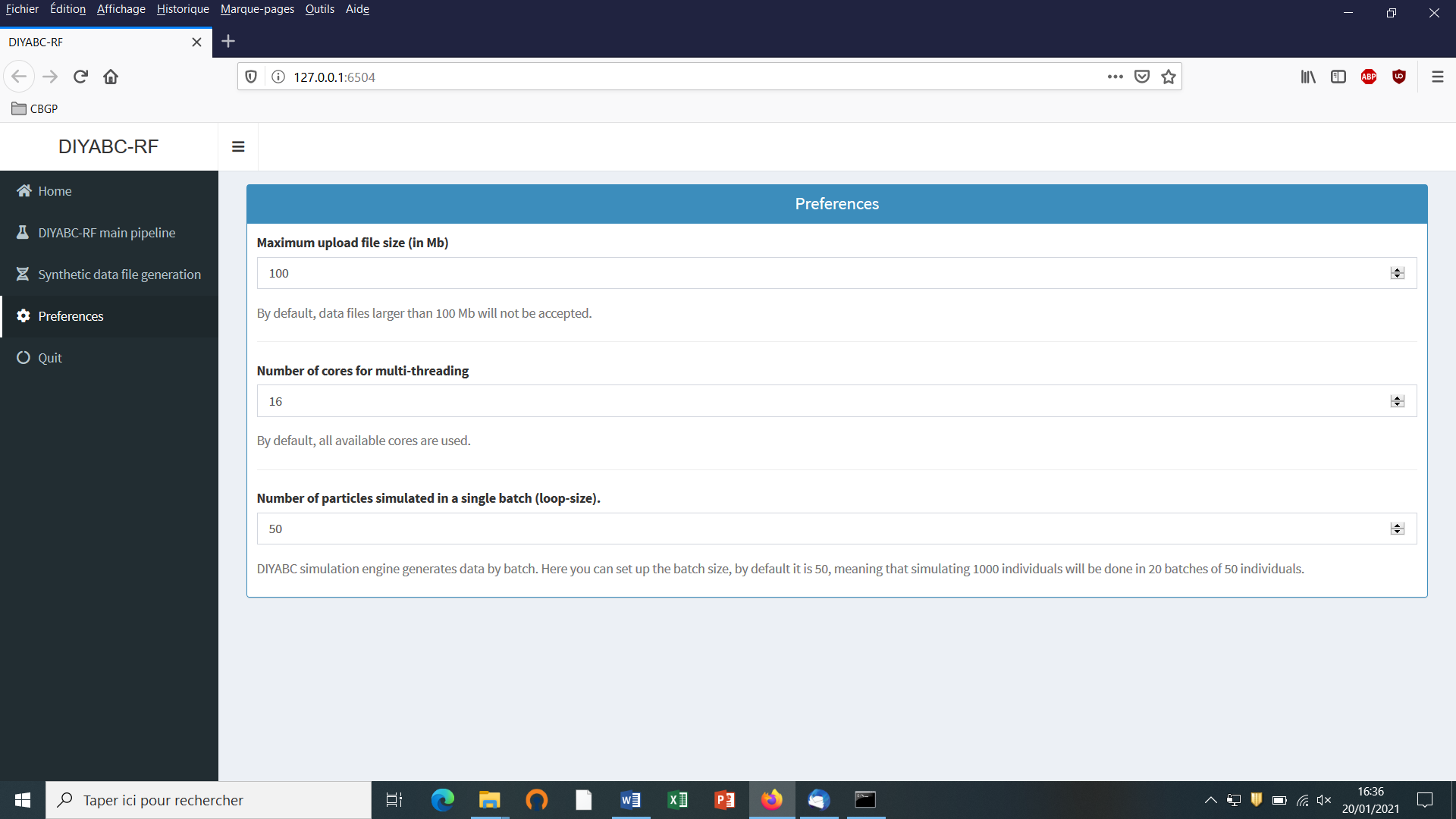
The different options proposed are self-meaning. Default values can be changed by the user. Note that the loop-size option corresponds to the number of simulated datasets distributed over all computer threads and stored in the RAM before writing them into the training set file (reftableRF.bin).

5.4 How to generate a new IndSeq SNP training set

5.4.1 Step 1: defining a new IndSeq project

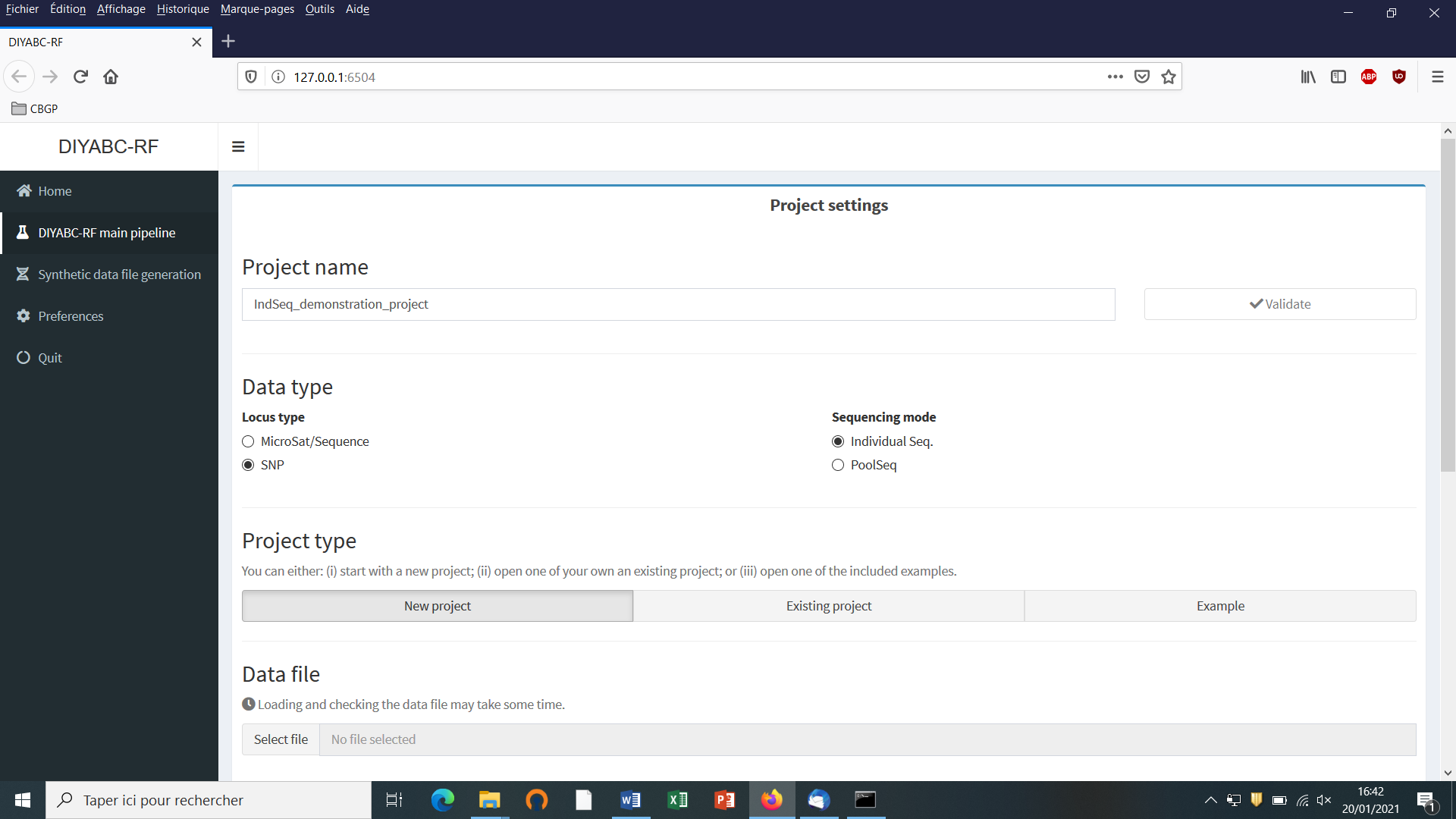
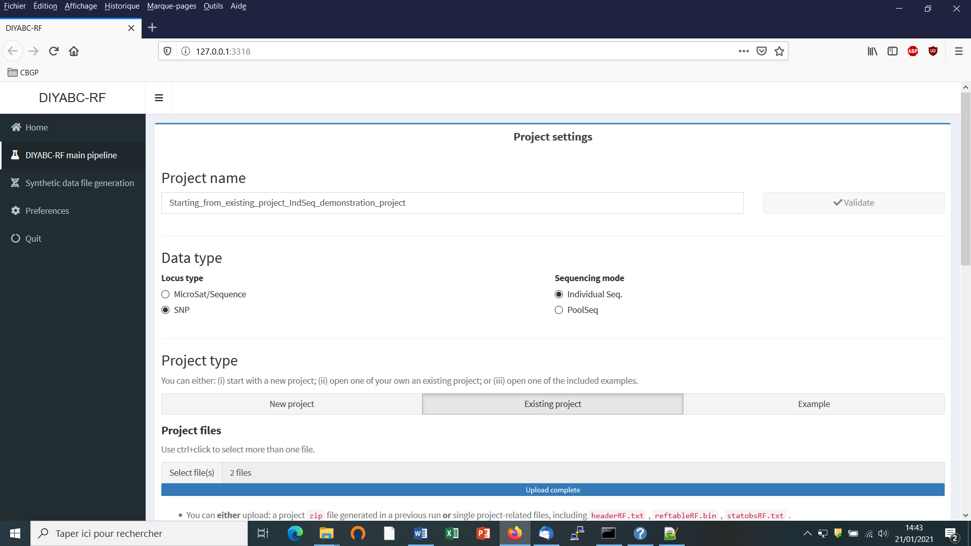
Defining a new project requires different steps which are not strictly the same whether the data are microsatellites/DNA sequences (MSS) or SNP (IndSeq or PoolSeq). Let’s start with an IndSeq SNP project. Click on the “Start” button in the middle of the Home panel (or on the “DIYABC-RF main pipeline” button). The following panel appears.

Enter a project name in the “Project name” window (here IndSeq_demonstration_project). Validate the project name.
Select the Data type including the locus type (Microsat/sequence or SNP) and the sequencing mode (for SNP only; IndSeq or PoolSeq). Here select SNP and Individual Seq.
Select the “New project” button as we want to implement a new project from scratch.

5.4.2 Step 2: choosing the data file

Choose a data file (an IndSeq format data file in this case) using the “Select file” browser (here INDSNP_sim_dataset_4POP_001.snp). A large size dataset might take some times to be uploaded and checked by the program. A short summary of the specificities of the loaded datafile appears: here the total number of loci (30000), the minimum allele frequency chosen for simulation (MAF=0.05), the sex ratio indicated by the user (NM=1NF), the total number of individuals and populations, the locus type and their corresponding numbers (A= autosomal, M=mitochondrial…; see section 7.1 for details about datafile format), and the number of available loci based on the MAF criterion (here 15617 <A>, as14383 loci, including 0 monomorphic loci, have been filtered out due to a MAF<5% by the program after scanning the proposed observed dataset).

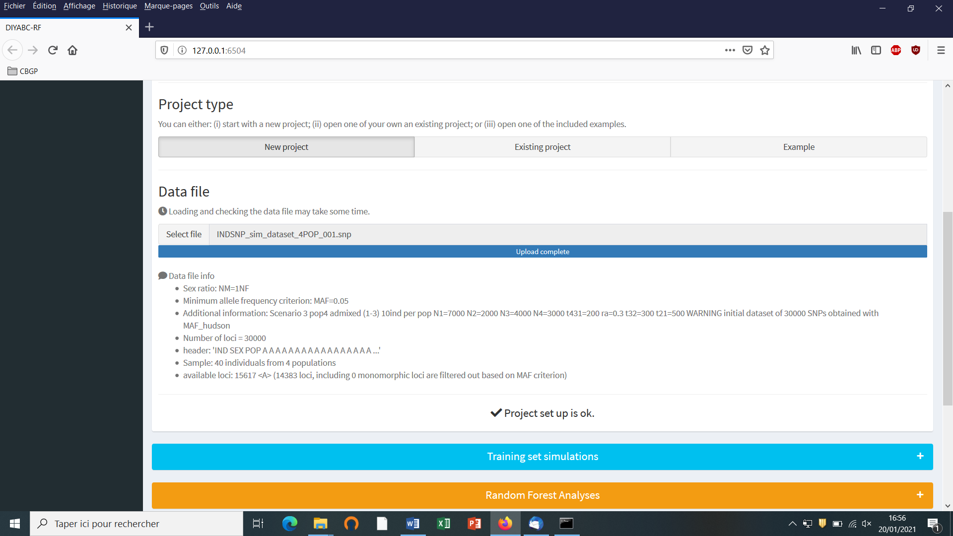
A “Project set up is ok” message appears at the bottom of the panel if all items have gone correctly. You can then go the next steps by clicking on the large blue color “Training set simulation” “+” button”. The following panel appears.

5.4.3 Step 3: Inform the historical model

Click on the “Add” button of the “Define historical models” section. The following panel appears:

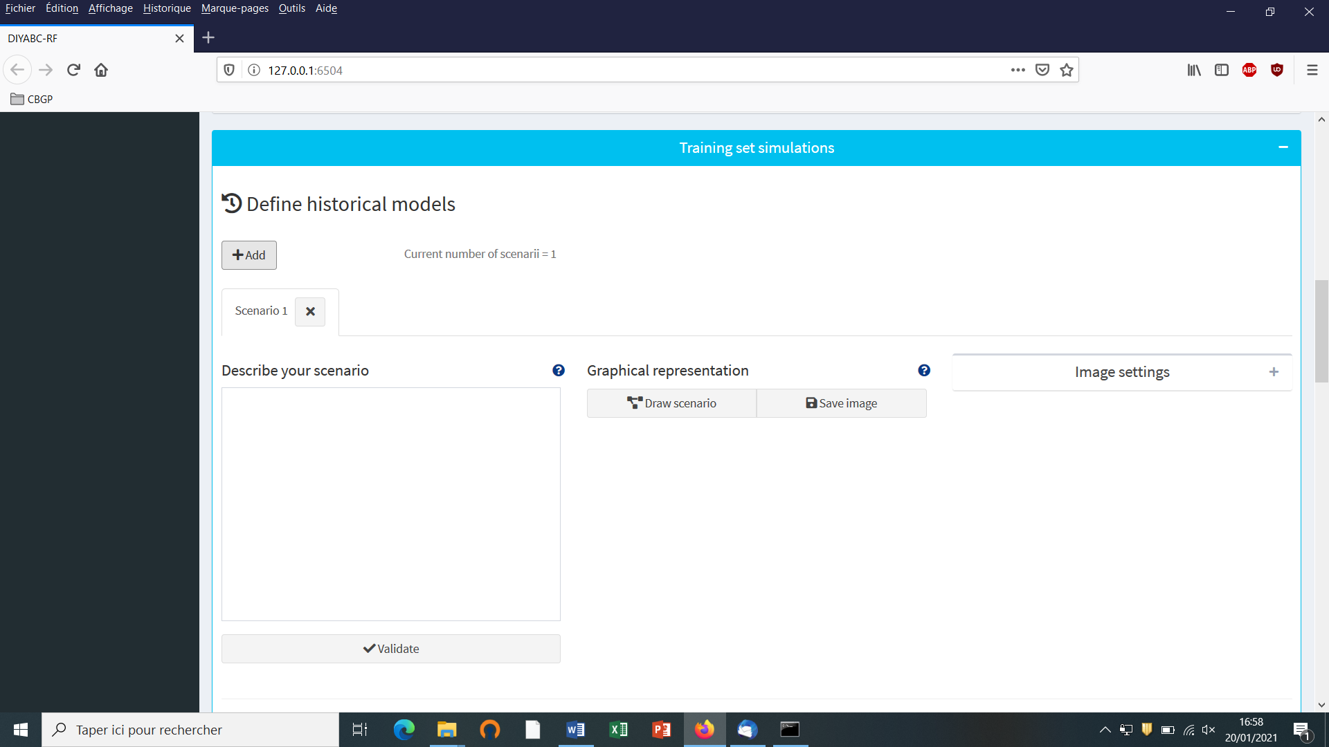
Write the code of a first scenario (scenario 1) in the edit window ”Describe your scenario” and click on the “Validate” button.

If we click on the “Draw scenario” button, the logic of the scenario is checked and if it is found OK, and if the scenario is draw-able, a graphical representation of the scenario appears. You can save it by clicking on the “Save image” button. Figures are saved in ‘fig’ sub-folder in the project directory. Possible extensions are: ‘eps’, ‘ps’, ‘tex’, ‘pdf’, ‘jpeg’, ‘tiff’, ‘png’, ‘bmp’, ‘svg’.

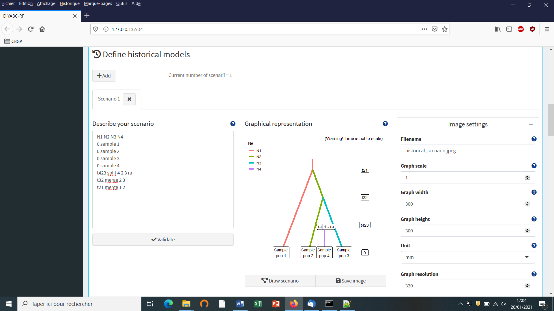
The “Priors and conditions” frame which appears below allows choosing the prior distribution of each parameter of the scenario. A parameter is anything in the scenario that is not a keyword (here sample, merge and split), nor a numeric value. In our example scenario, parameters are hence: N1, N2, N3, N4, ra, t21, t32 and t423. We choose a uniform distribution and change the min and max values (100 and 10000 for N values - 10 and 1000 for t values; see panel below).

In our example, we also need to specify conditions for the priors on t21, t32 and t432 such that t21>t32 and t32>t423.

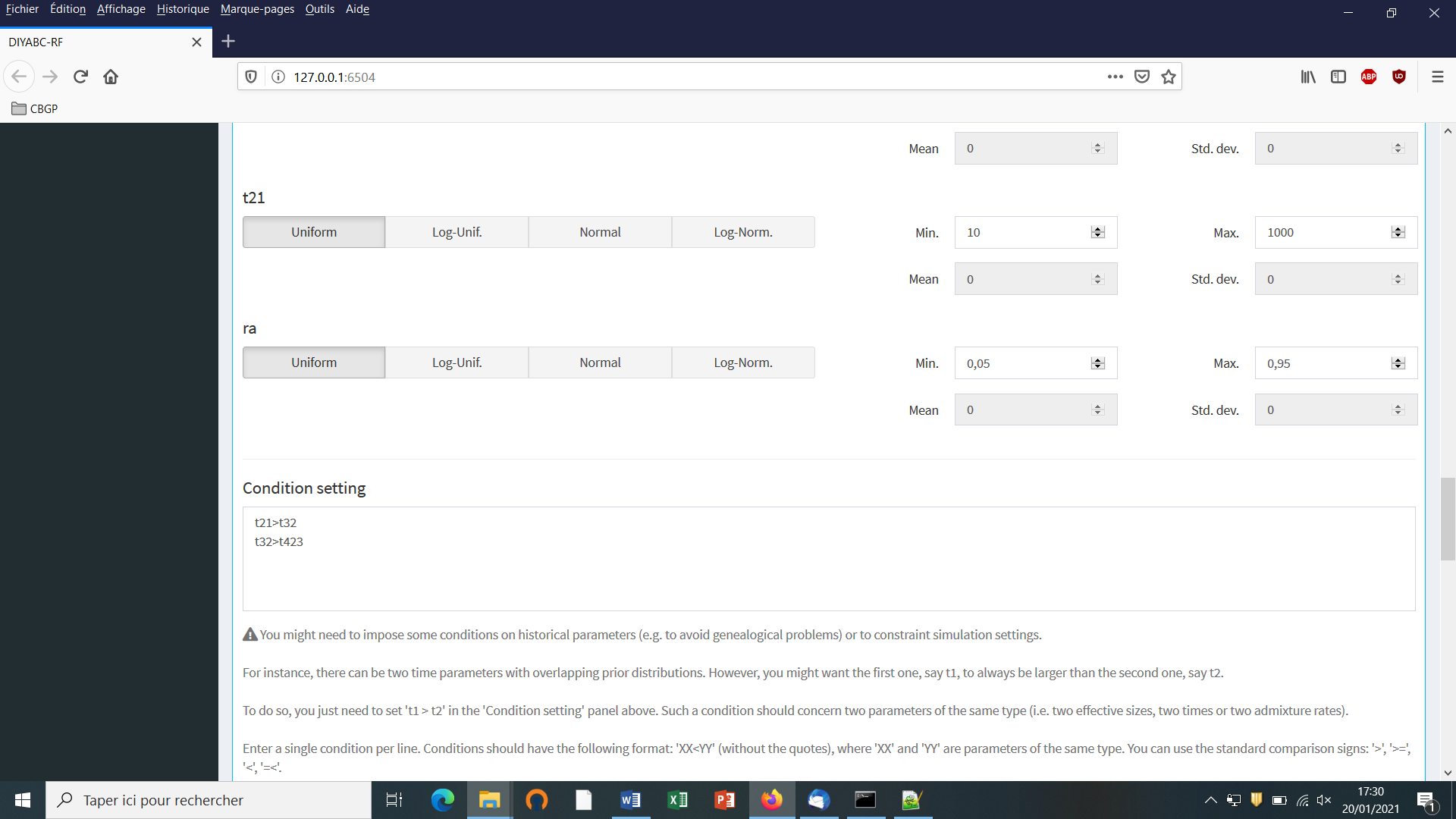
To do this we write t21>t32 and t32>t432 on two successive lines in the “Condition setting” frame. As noted in the panel, conditions should have the following format: XX<YY. where ‘XX’ and ‘YY’ are parameters of the same type. You can use the standard comparison signs: ‘>’, ‘>=’, ‘<’, ‘=<’. It is worth stressing that the omission of such conditional constraints on merge times (cf. a population needs to exist in the past to allow coalescence events in it) is one of the most frequent implementation error made by DIYABC-RF users. If forgotten a message “Error in simulation process: check your scenarios, priors and conditions” appears. Note that the occurrence of a too large number of time conditional constraints within a scenario may substantially slow down simulations as a valid t parameter vector will be retain and run only once all conditions are fulfilled.

We then can add some other scenarios in additional windows by clicking on the button “Add” (one or several times if one wants to add a single or several other scenarios). In the present example, we simulate datasets from six different scenarios that we want to compare (see Collin et al. 2020 example based on pseudo-observed datasets for details); hence the six scenario windows that we have completed with instructions for each one. For the last sixth scenario the panel looks like this:

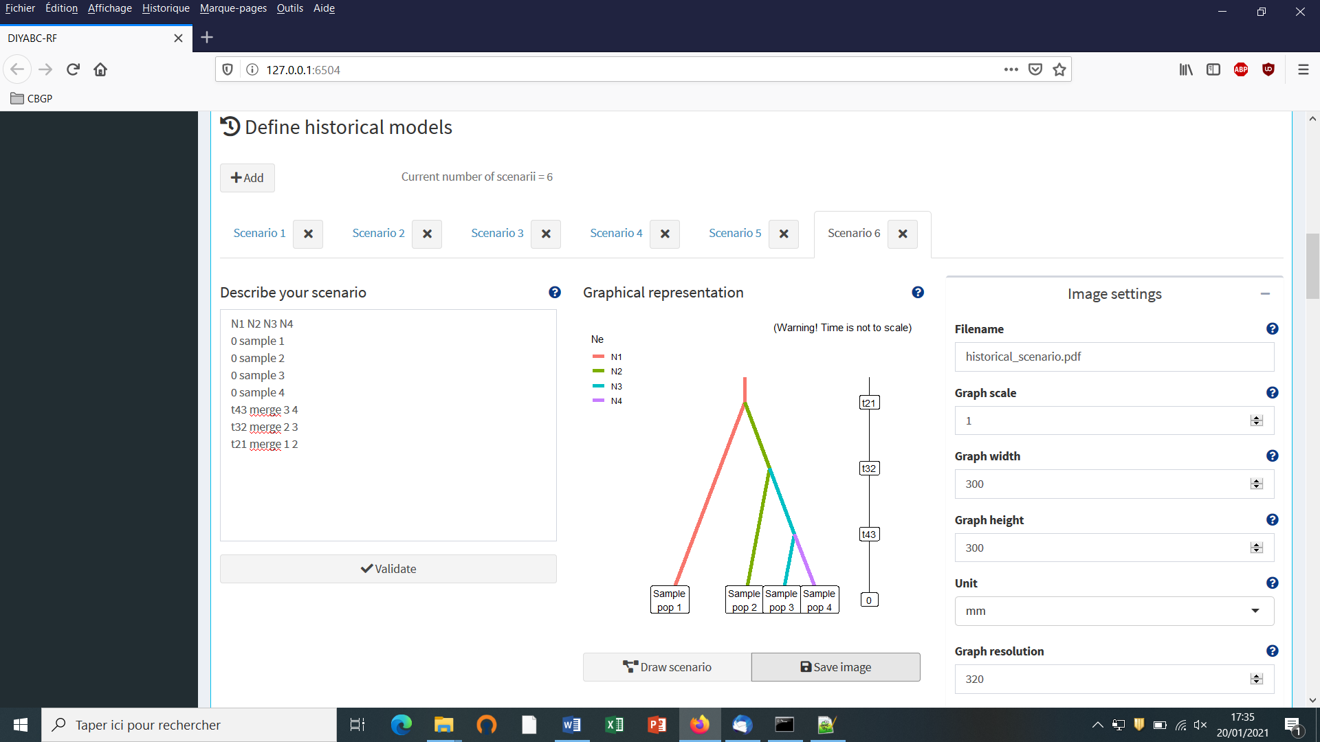
You need to complete time conditions for the six scenarios by writing t21>t32, t42<t21, t43<t32, t32>t423, t431<t32 and t421<t21 on successive lines in the “Condition setting” frame.

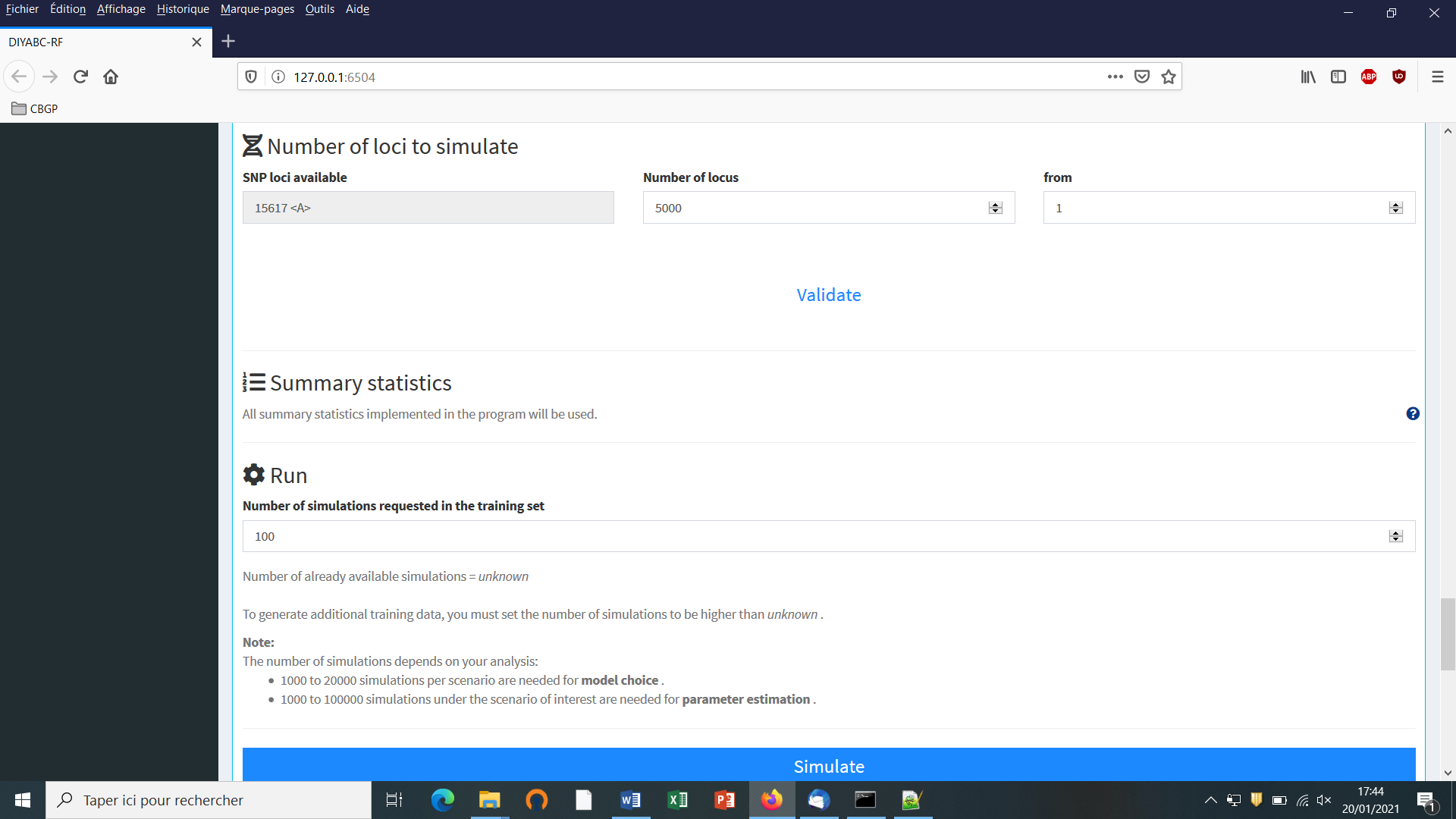
5.4.4 Step 4: Inform number of loci to simulate (and chromosome type)

Choose the number of SNP locus that you want to simulate for each chromosome type define in the data file (A for autosomal diploid loci, H for autosomal haploid loci, X for X-linked or haplo-diploid loci, Y for Y-linked loci and M for mitochondrial loci; see section 7.1.1). Here we have only type <A> SNP loci. According to our own experience, analyzing (evolutionary neutral) scenarios using 5000 to 20000 SNP loci is sufficient to obtain robust results. In this example, we choose to consider simulations based on a subset of 5000 SNP loci (with <MAF=0.05> as indicated previously in the headline of the observed dataset file) taken in order from the first SNP locus of the data file (users may want to change this stating point), by replacing 30000 by 5000 in the corresponding frame. Click on the button “Validate”.

It is worth stressing that choosing a subset of 5000 SNP loci taken from the SNP locus 5001 of the data file would lead to a training set generated from a set of 5000 loci completely independent from the previous one. Generating by this way different training sets is a way to process independent analyses of a given dataset (a sufficiently large number of SNP loci available in the observed dataset is obviously needed to do that).

5.4.5 Step 5: Summary statistics

In the present version of the program, all available summary statistics are computed as mentioned in the interface below the “Summary statistics” item (see previous panel-copy) and as detailed when clicking on the button “?” on the right:

For both IndSeq and PoolSeq SNP loci, the following set of summary statistics has been implemented.

1. Proportion of monomorphic loci for each population, as well as for each pair and triplet of populations (ML1p, ML2p, ML3p)

Mean and variance (over loci) values are computed for all subsequent summary statistics.

2. Heterozygosity for each population (HW) and for each pair of populations (HB)

3. FST-related statistics for each population (FST1), for each pair (FST2), triplet (FST3), quadruplet (FST4) and overall (FSTG) populations (when the dataset includes more than four populations)

4. Patterson’s f-statistics for each triplet (f3-statistics; F3) and quadruplet (f4-statistics; F4) of populations

5. Nei’s distance (NEI) for each pair of populations

6. Maximum likelihood coefficient of admixture (AML) computed for each triplet of populations.

Note the short code name for each type of summary statistics (MLP1p, HW, FST2, F3,…). Such code names of statistics (plus the suffix m and v for mean and variance over loci, respectively; see section 2.6.3) will be used in most files produced by the program, including the key files headerRF.txt, reftableRF.bin and statobsRF.txt.

5.4.6 Step 6: Simulate the training set

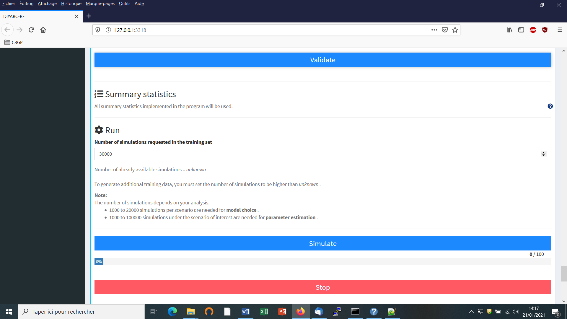
You can access the “training set simulation” module by clicking on the corresponding + button on the far right of the box blue title bar “Training set simulation”. The following “Run” panel appears.

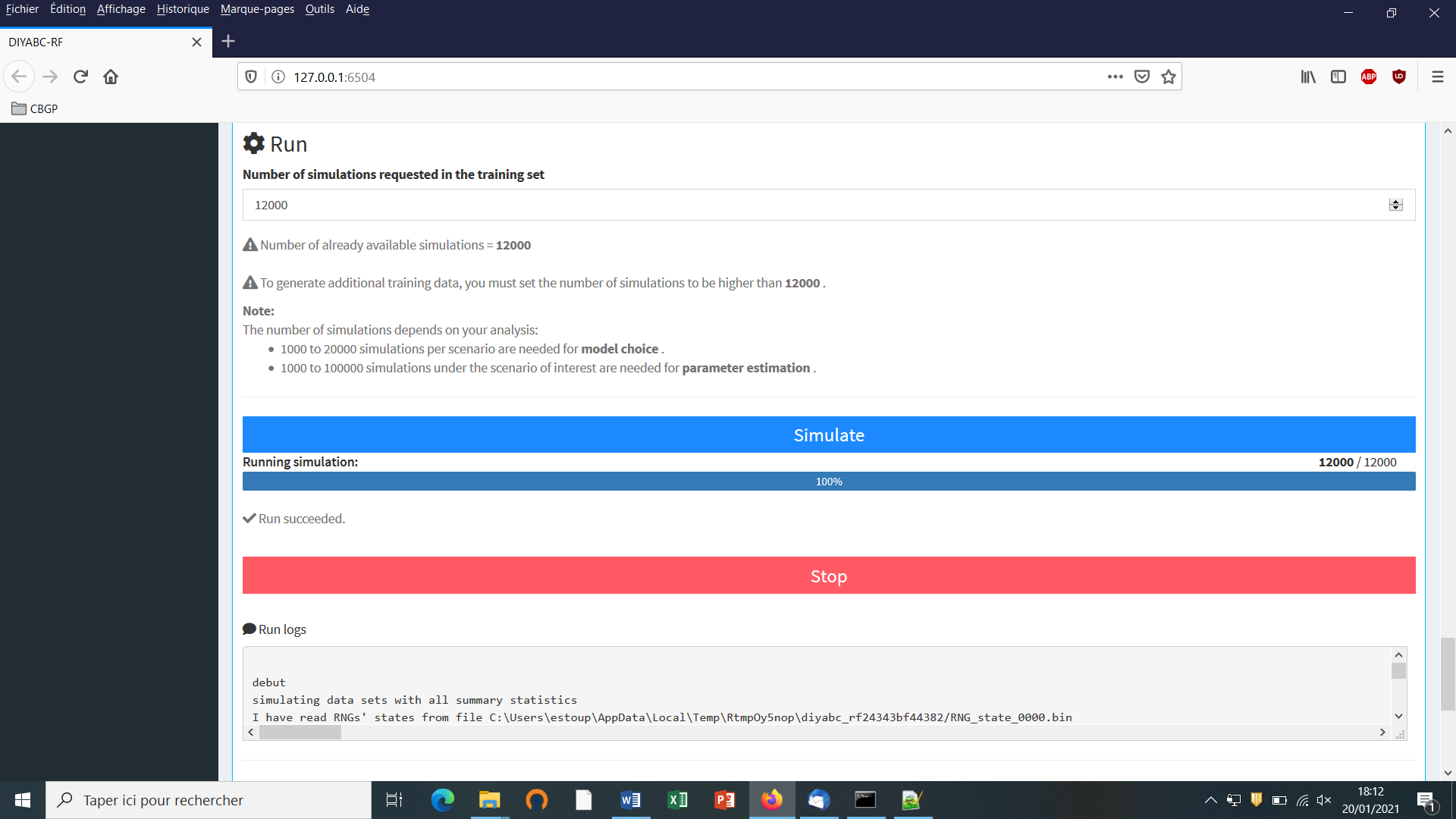
Indicate the required number of datasets to simulate in the training set: we here change the default value of 100 into 12000 (in order to simulate 2000 datasets for each of the six scenarios)
Launch the generation of the simulated datasets of the training set by clicking on the large blue color button “Simulate”. The number of datasets already simulated is given in the “Running simulation” progress bar below.

You can stop the generation of simulated datasets by clicking on the “STOP” button. Both a “Run succeeded” message appears when all requested simulations have been processed.
Do not forget to click on the “Save” button in the “Project administration” lower panel (see panel below) to implement and save a concatenated zip file including various input and output files (see section 7 for a description of the content of some of those files) on your computer. The name of the implemented/saved concatenated .zip file is the one given at the start in the “Project name” window (here IndSeq_demonstration_project).

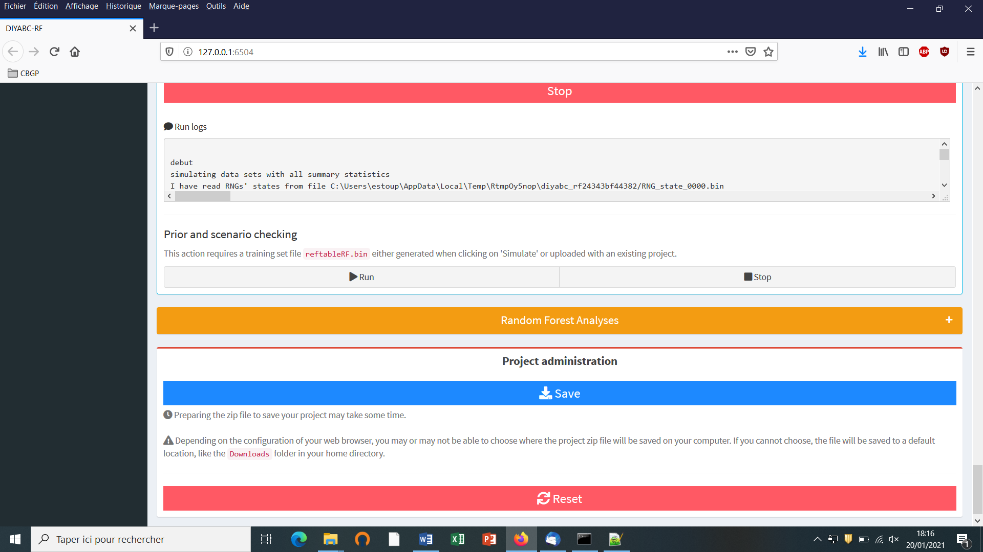
Warning: The “Reset” button at the very bottom part of the “Project administration” panel restart the pipeline from scratch removing all configurations previously set up and all data and result files generated.

5.4.7 Step 7:Prior-scenario checking PRE-ANALYSIS (optional but recommended)

Before performing a full ABC-RF analysis on a large size training set, we advise using the prior-scenario checking option on a training set of small size (e.g. including 500 to 1000 simulated dataset per scenarios). As a matter of fact, this pre-analysis option is a convenient way to reveal potential mis-specification of models (scenarios) and/or prior distributions of parameters (and correct it). This action requires a training set file (reftableRF.bin) and a statobsRF.txt file either generated when clicking on the “Simulate” button or uploaded with an existing project. When clicking on the “Run” button of the “Prior and scenario checking” option (see previous panel copy) the program will generate two specific outputs:

A Principal Component Analysis (PCA) representing on 2-axes plans the simulated dataset from the training set and the observed dataset as graphical output. Note that this figure is somewhat similar in its spirit to the graphical output LDA_training_set_and_obs_dataset.png obtained when running the scenario choice option in “Random Forest Analyses”. The latter output is different, however, as it corresponds to the projection of the datasets from the training set linear discriminant analysis (LDA) axes (see section 7.3 for details).
A numerical output file, named pcaloc1_locate.txt, which includes for each summary statistics and for each scenario, the proportion of simulated data (considering the total training set) that have a summary statistics value below the value of the observed dataset. A star indicates proportions lower than 5% or greater than 95% (two stars, <1% or >1%; three stars, <0.1% or >0.1%). The presence of such star symbols is a sign of substantial mismatch between the observed dataset and the simulated datasets. The latter numerical results can help users to reformulating the compared scenarios and/or the associated prior distributions in order to achieve some compatibility (see e.g. Cornuet et al. 2010). If only a few stars are observed at a few summary statistics for one or several scenarios, one can conclude that prior-scenario conditions are suitable enough to further process Random Forest analysis, and this potentially on a training set including more simulated datasets.

5.5 How to generate a new PoolSeq SNP training set

Follow the same steps described in section 5.4 for IndSeq SNPs.

Step 1: Defining a new PoolSeq SNP project  see section 5.4.1

Click on the “Start” button of the home screen. Select SNP as project type and PoolSeq as sequencing mode

Step 2: Choosing the data file  see section 5.4.2 and select a dataset file characterized by a PoolSeq format (format detailed in section 7.1.2).
Step 3: Inform the Historical model  see section 5.4.3
Step 4: Inform chromosome type and number of loci  see section 5.4.4

Note: The panel for PoolSeq SNPs is simpler than for IndSeq SNPs because PoolSeq SNPs are considered as located on autosomal chromosomes only.

Step 5: Summary statistics:  see section 5.4.5
Step 6: Simulate the training set  see section 5.4.6
Step 7 (optional but recommended): Prior-scenario checking PRE-ANALYSIS  see section 5.4.7

5.6 How to generate a new microsatellite (and/or DNA sequence) training set

Follow the same steps described in section 5.4 for IndSeq SNPs.

Step 1: Defining a new or microsatellites/DNA sequences project  see section 5.4.1

Click on the “Startt” button of the home screen. Select Microsat/Sequences as project type (not any sequencing mode is needed)

Step 2: Choosing the data file  see section 5.4.2 and select a dataset file characterized by a Microsatellite and/or DNA Sequences format (format detailed in section 7.1.3).
Step 3: Inform the Historical model  see section 5.4.3
Step 4: The panel “Inform chromosome type and number of loci” is replaced by the panel “Inform the genetic model”  see details below in section 5.6.1

Step 5: Summary statistics: different sets of summary statistics are computed as compared to SNP summary statistics  see details below in section 5.6.2
Step 6: Simulate the training set  see section 5.4.6
Step 7 (optional but recommended): Prior-scenario checking PRE-ANALYSIS  see section 5.4.7

5.6.1 Step 4: Inform the genetic model

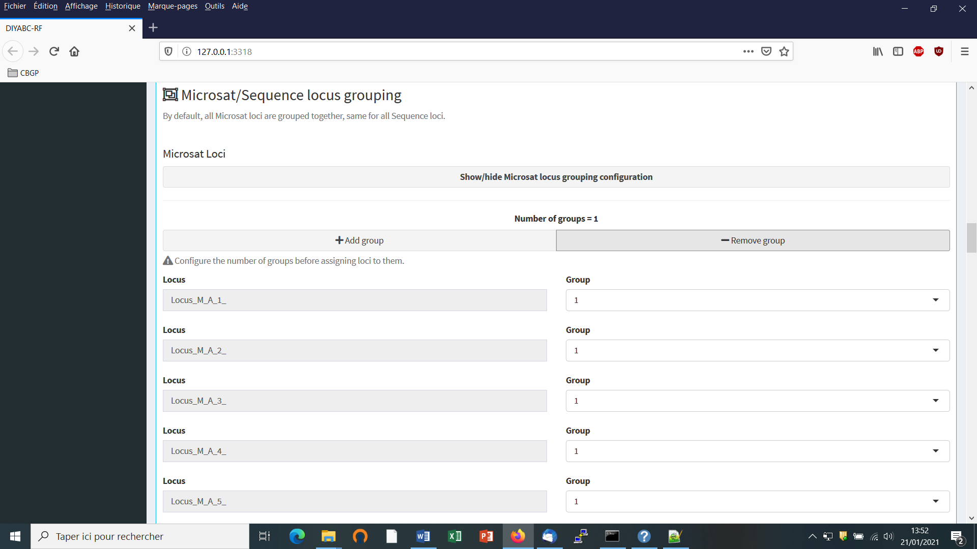
For microsatellite markers: Informing the genetic model can be done using the following panels (implemented here from a toy example including microsatellites + DNA sequences named TOY_EXAMPLE2_microsatellites_DNAsequence_two_pops_ancient_admixture; see section 10. “TOY EXAMPLES” for details about this toy example).

First: define the number of groups of markers (a group been defined by different mutational modalities). By default, all microsatellite loci are grouped together, same for all DNA sequence loci. If you want to define more than a single group then configure the number of groups (cf button “Add group”) and then assign each locus to one of those groups using the Group arrow on the right.

Second: define the motif size and continuous range of motif variation. By default, all microsatellite loci are supposed to be dinucleotidic (motif = 2) with a range of 40.

It is worth stressing that the values for motif size and allelic range are just default values and do not necessarily correspond to the actual microsatellite observed dataset. The user who knows the real values for its data is required to set the correct values at this stage. If the range is too short to include all values observed in the analyzed dataset, a message appears in a box asking to enlarge the corresponding allelic range. Note that the allelic range is measured in number of motifs, so that a range of 40 for a motif length of 2 bp means that the difference between the smallest and the longest alleles should not exceed 80 bp. It is worth stressing that the indicated allelic range (expressed in number of continuous allelic states) corresponds to a potential range which is usually larger than the range observed from the analyzed dataset (cf. all possible allelic states have usually not been sampled). In practice it is difficult to assess the actual microsatellite constraints on the allelic range; to do that one needs allelic data from several distantly related populations/sub-species as well as related species which is rarely the case(see Pollack et al. 1998; Estoup et al. 2002). We achieved a meta-analysis from numerous primer notes documenting the microsatellite allelic ranges of many (i.e. > 100) different species (and related species). We used the corrective statistical treatment on such data proposed by (Pollack et al. 1998). Our results pointed to a mean microsatellite allelic range of 40 continuous states (hence the default allelic range value of 40 mentioned in the program). We also found, however, that range values greatly varied among species and among loci within species (unpublished results). We therefore recommend the following pragmatic choice when considering the allelic range of your analyzed microsatellite dataset: (i) if the difference in number of motif of your locus is < 40 motifs in the analyzed dataset then leave the default allelic range value of 40. (ii) if the difference in number of motif of your locus is >40 motifs in your dataset then take Max_allele_size $-$ Min_allele_size)/motif size + say 10 additional motifs to re-define the allelic range of the locus in the corresponding DIYABC-RF panel (e.g. (200 nu $-$ 100 nu)/2 + 10 = 50 + 10 = 60 as allelic range).

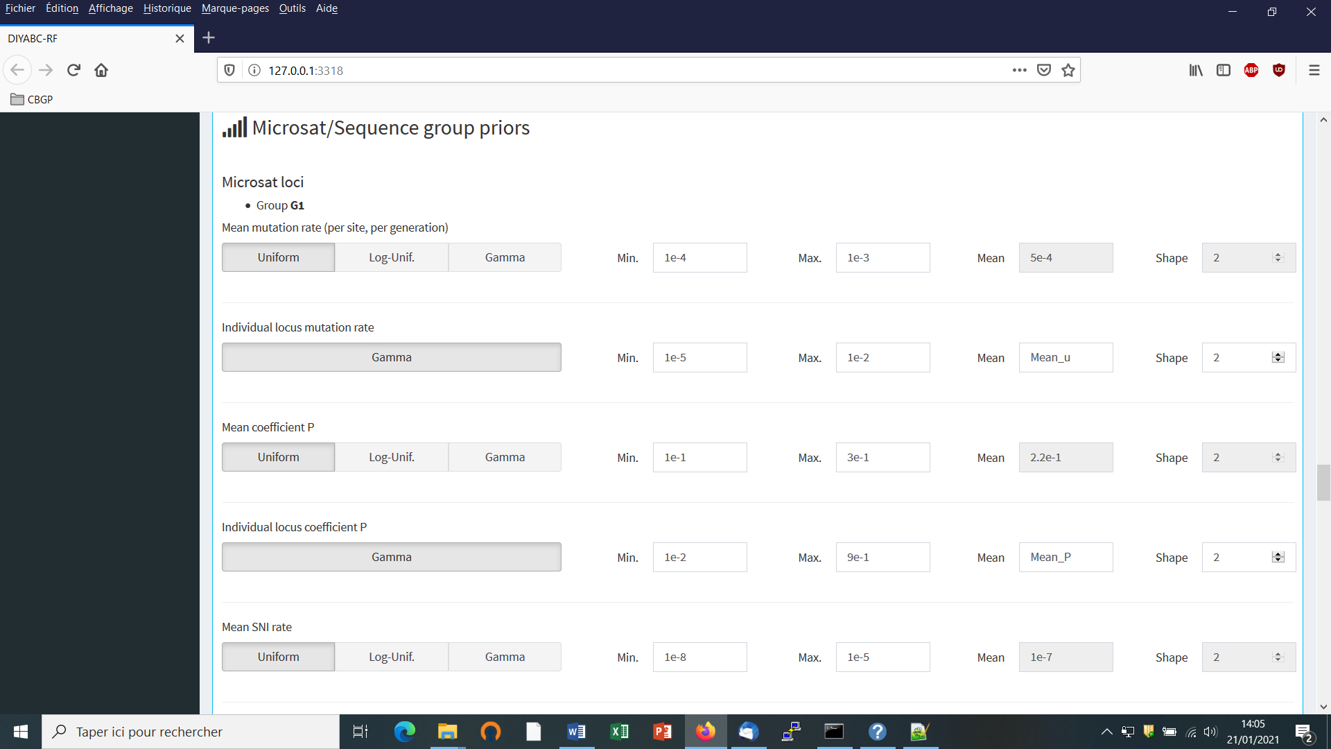
Third: adjust the prior specificities of mutational modalities as you want using the corresponding buttons in the panel below. Otherwise keep the default values as the latter have been reported for many eukaryote species (e.g. Estoup et al. 2002; but see Fraimout et al. 2017).

For DNA sequence markers: Informing the genetic model can be done using the following panels (implemented here from the same toy example as above).

We need to define at least one group of DNA sequence loci.

Suppose that we want all DNA sequence loci in the same group because we consider that they all have similar mutational modalities. We then put “2” in the button “Group” for all loci (Group 1 is for the previous microsatellite markers). Otherwise you can associate some loci to additional groups (after clicking on the button “Add group”) if you consider that such loci have different mutational modalities (for instance here Locus_S_M_16_ corresponding to a sequence of mitochondrial DNA).
Adjust the prior specificities of mutational modalities (for the different DNA sequence groups you have defined previously) using the corresponding buttons in the panel below. Otherwise keep the default values as the latter have been reported for many eukaryote species (e.g. Cornuet et al. 2010).

The default values are indicated in the panel. Note that the default mean mutation rate is not suited to mitochondrial DNA which generally evolves at a faster rate than nuclear DNA (Haag-Liautard et al., 2008). So we set its value to 10^-8. For all other mutation model parameters, one can just keep the default values. See section 2.4.2 “DNA sequence loci” for details about the mutation models proposed for DNA sequences.

Before launching a run to simulate the training set, do not forget to validate your microsatellite and/or DNA settings by clicking on the blue-color button “Validate”. Indicate the number of simulations in the corresponding button (here 30000) and click on the button “Simulate” to launch the simulation of the training set.

5.6.2 Step 5: Summary statistics

In the present version of the program, all available summary statistics are computed as mentioned in the interface below the “Summary statistics” item (see previous panel-copy) and as detailed when clicking on the button “?” on the right:

For microsatellite loci

The following set of summary statistics has been implemented.

Single sample statistics:

1. mean number of alleles across loci (NAL)

2. mean gene diversity across loci (HET)

3. mean allele size variance across loci (VAR)

3. mean M index across loci (MGW)

Two sample statistics:

1. mean number of alleles across loci (two samples) (N2P)

2. mean gene diversity across loci (two samples) (H2P)

3. mean allele size variance across loci (two samples) (V2P)

${3.F}_{ST}$ between two samples (FST)

4. mean index of classification (two samples) (LIK)

5. shared allele distance between two samples (DAS)

6. distance between two samples (DM2)

Three sample statistics:

1. Maximum likelihood coefficient of admixture (AML)

For DNA sequence loci

The following set of summary statistics has been implemented.

Single sample statistics:

1. number of distinct haplotypes (NHA)

2. number of segregating sites (NSS)

3. mean pairwise difference (MPD)

4. variance of the number of pairwise differences (VPD)

5. Tajima’s D statistics (DTA)

6. Number of private segregating sites (PSS)

7. Mean of the numbers of the rarest nucleotide at segregating sites (MNS)

8. Variance of the numbers of the rarest nucleotide at segregating sites (VNS)

Two sample statistics:

1. number of distinct haplotypes in the pooled sample (NH2)

2. number of segregating sites in the pooled sample (NS2)

3. mean of within sample pairwise differences (MP2)

4. mean of between sample pairwise differences (MPB)

${5.F}_{ST}$ between two samples (HST)

Three sample statistics:
1. Maximum likelihood coefficient of admixture (SML)

5.7 How to work from an “Existing project” (for any type of markers)

Working from an existing project is particularly appealing when one wants to:

(i) objective 1: simply add more simulations in the training set of the reftableRF.bin of an existing project without changing anything in the headerRF.txt.

(ii) objective 2: use the headerRF.txt content of an existing project as a base to generate a new headerRF.txt file including different changes for instance in the scenarios formulated, in the definition of priors, the number of loci to simulate…

Let’s consider that one wants to work from the IndSeq_demonstration_project previously generated (and including a training set with 12000 simulation records) as described in the above section 5.4.

Click on the “Start” button in the middle of the Home panel. The following panel appears.

Enter a project name in the “Project name” window (here “Starting_from_existing_project_IndSeq_demonstration_project”) and validate the project name.
Select the project type (Microsat/sequence or SNP) and the sequencing mode (for SNP only; IndSeq or PoolSeq). As we will start from a pre-existing IndSeq project, select SNP and Individual Seq.
Click on the “Existing project” button of the ”Project type” item as we want to work from an existing project.
Use the browser of the “Project files” item to select key files in the Existing project directory (here a directory named “IndSeq_demonstration_project”). Key files are headerRF.txt (mandatory), reftableRF.bin (if one simply wants to add more simulations in the training set of the reftableRF.bin of an existing project without changing anything in the headerRF.txt cf. objective 1 above), and statobsRF.txt (optional). If the objective 2 is concerned then only the file headerRF.txt is needed (avoid loading the reftableRF.bin file as the latter might not be in accordance with the new headerRF.txt file and the associated simulated data that you will generate).

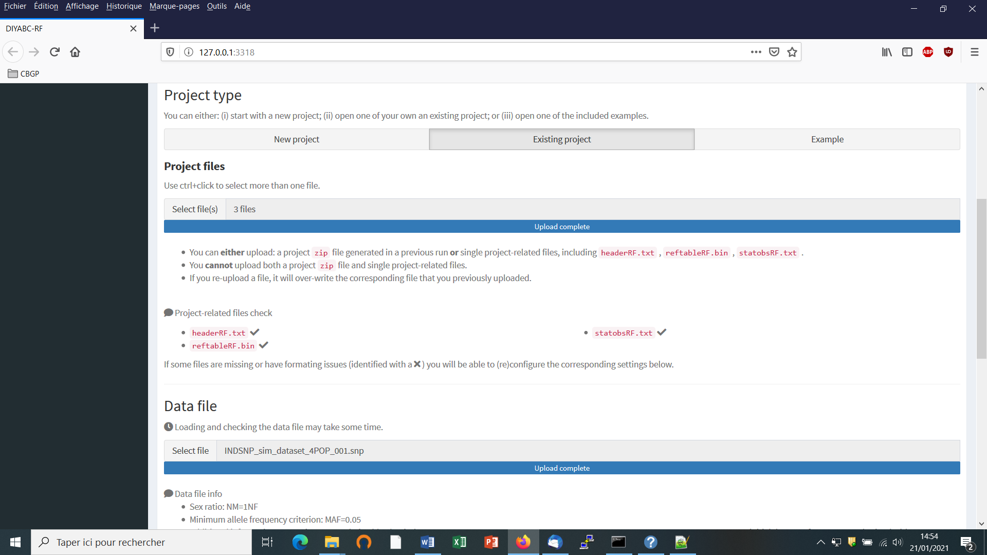
Browse and choose a data file (an IndSeq format data file in this case) in the “Data file” window (here INDSNP_sim_dataset_4POP_001.snp). A short summary of the specificities of the loaded datafile appears: here the total number of loci (30000), the minimum allele frequency chosen for simulation (MAF=0.05), the sex ratio indicated by the user (NM=1NF), the total number of individuals and populations, and finally the locus type and their corresponding numbers (A= autosomal, M=mitochondrial,…), including information regarding the number of loci available after applying the MAF (or MRC) criterion; see section 7.1 for details about data file format.
A “Project set up is ok” message appears at the bottom of the panel if all items have gone correctly. You can then go the next steps by clicking on the large blue color “Training set simulation” “+” button”. The following panel appears.

The panel displays all information included in the headerRF.txt file (historical models, priors and conditions, number of SNP loci to simulate). Warning: such information cannot be changed.

To change information in the headerRF.txt (cf. **objective 2**) click on the “Edit configuration” button located at the top of the panel and changes for instance the scenarios formulated, the definition of priors, the number of loci to simulate etc. In this case a new reftableRF.bin file will be generated from scratch following the instruction included in the newly generated headerRF.txt file.

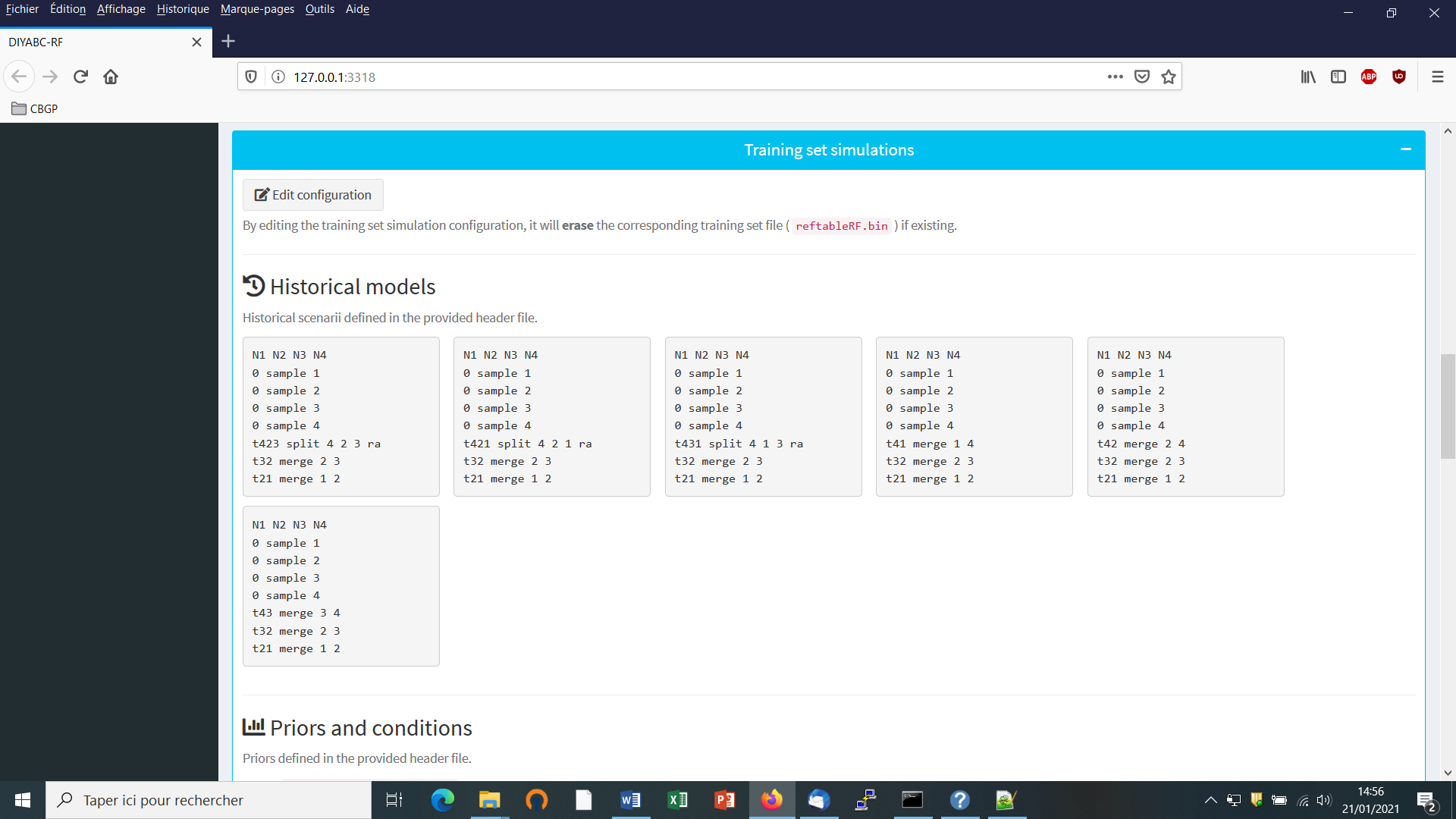
Following objective 1, you can launch new simulations that will be added to those already present in the pre-existing training set (i.e. reftableRF.bin file). As we have already 12000 simulations in the initial reftableRF.bin file we put the number of simulation to a number > 12000 (here 24000 to double the number of simulated data). Then click on the large blue color button “Simulate”.

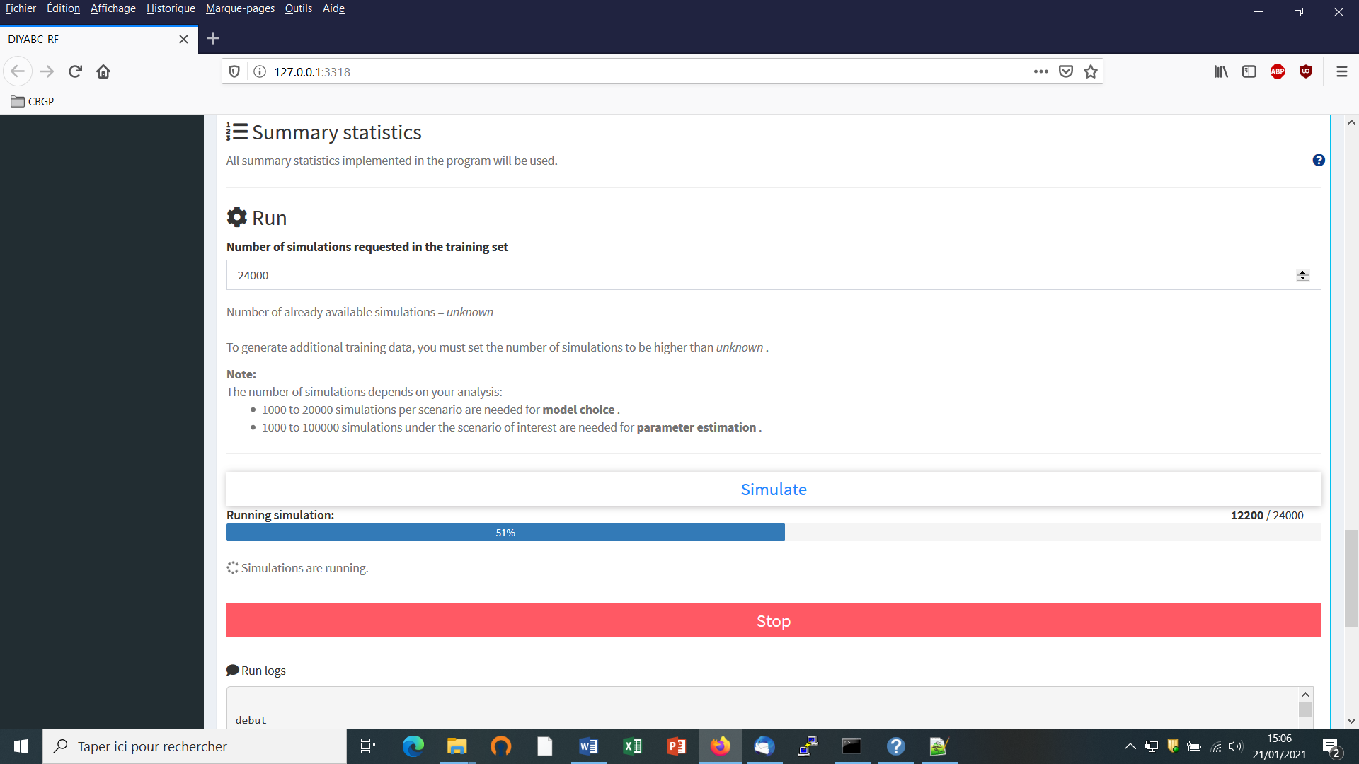
You can stop the generation of simulated datasets by clicking on the “STOP” button. A “Run succeeded” message appears when all requested simulations have been processed.

Do not forget to click on the “Save” button in the “Project administration” lower panel to implement and save a concatenated zip file including various input and output files (see section 7 for a description of the content of some of those files) on your computer. The name of the implemented/saved concatenated .zip file is the one given at the start in the “Project name” window (here Starting_from_existing_project_IndSeq_demonstration_project).

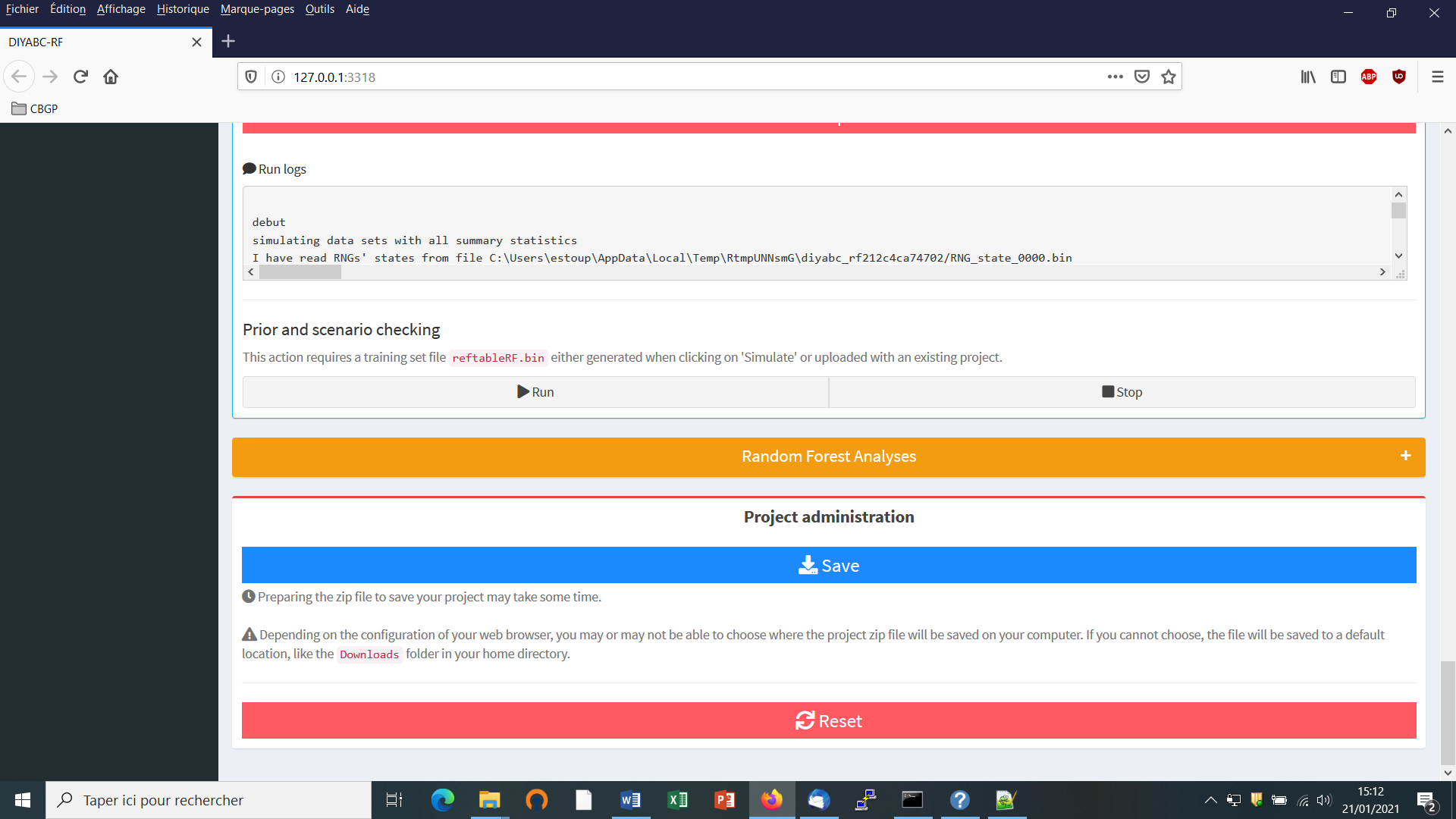
You might also want to launch the optional but recommended option “Prior and scenario checking”. For details see section 5.4.7.
Warning: The button “Reset” at the very bottom part of the “Project administration” panel restart the pipeline from scratch removing all configurations previously set up and all data and result files generated.

6. PERFORMING RANDOM FOREST ANALYSES

6.1 Files needed

Four files are needed at this stage:

the file headerRF.txt which describes the full settings of the generation of the training set
the training set file reftableRF.bin (generated from the headerRF.txt file),
the file statobsRF.txt which corresponds to the values of the summary statistics computed for the observed dataset and which was generated when producing the headerRF.txt and reftableRF.bin files.
Warning: although not necessary per se for Random Forest analyses (as the later only need the statobsRF.txt file as data point to analyze), the observed (here IndSeq SNP) data file has to be loaded too.
It is worth stressing that these files are: (i) already available following an in-course (and terminated) training set simulation or (ii) they can be selected and loaded independently by clicking on the “Existing project” button and using the ”Project files” and “Data file” browsers.

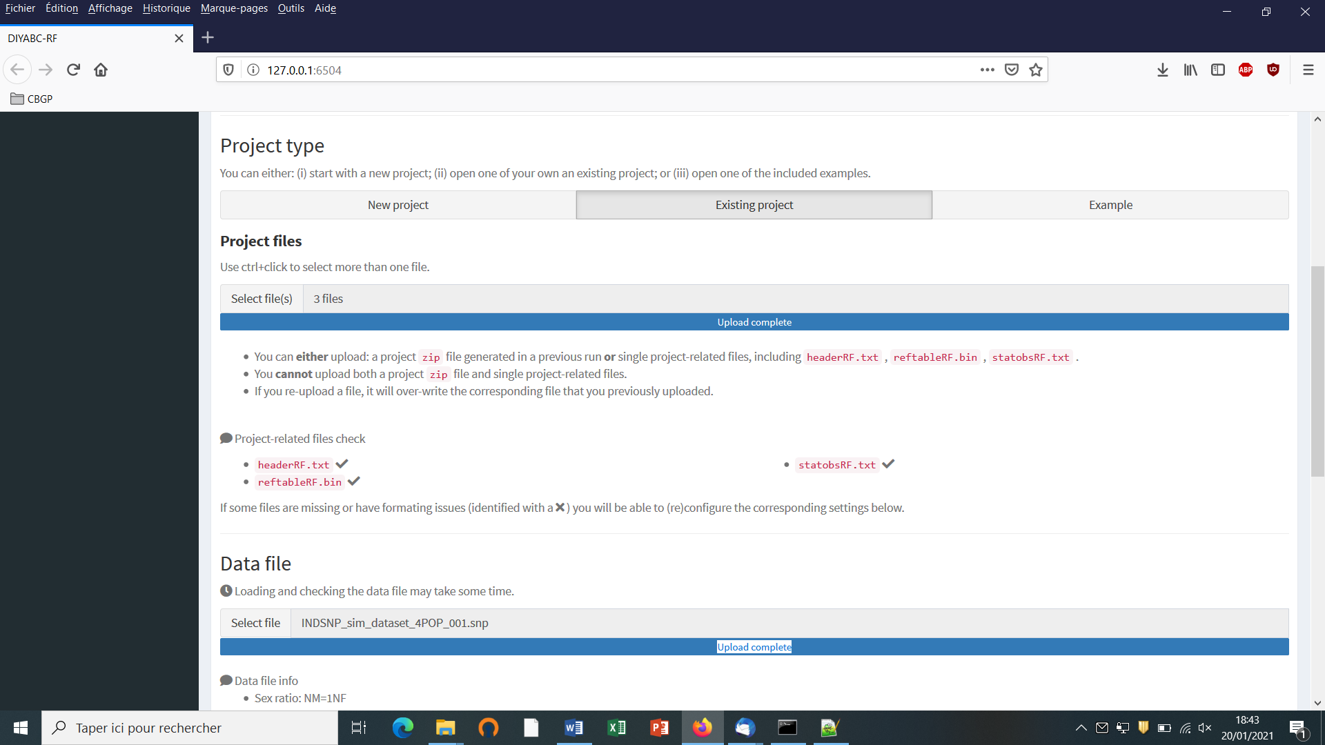
6.2. Scenario choice analysis

Click on the large orange color “Random Forest Analyses” button (“+” on the right).
Click on the button “Check input”: useful information about the training set (cf. reftableRF.bin file) content is provided (nbr of scenarios, total nbr of simulated datasets, nbr of simulated dataset available per scenario, nbr of parameters, nbr of summary statistics).

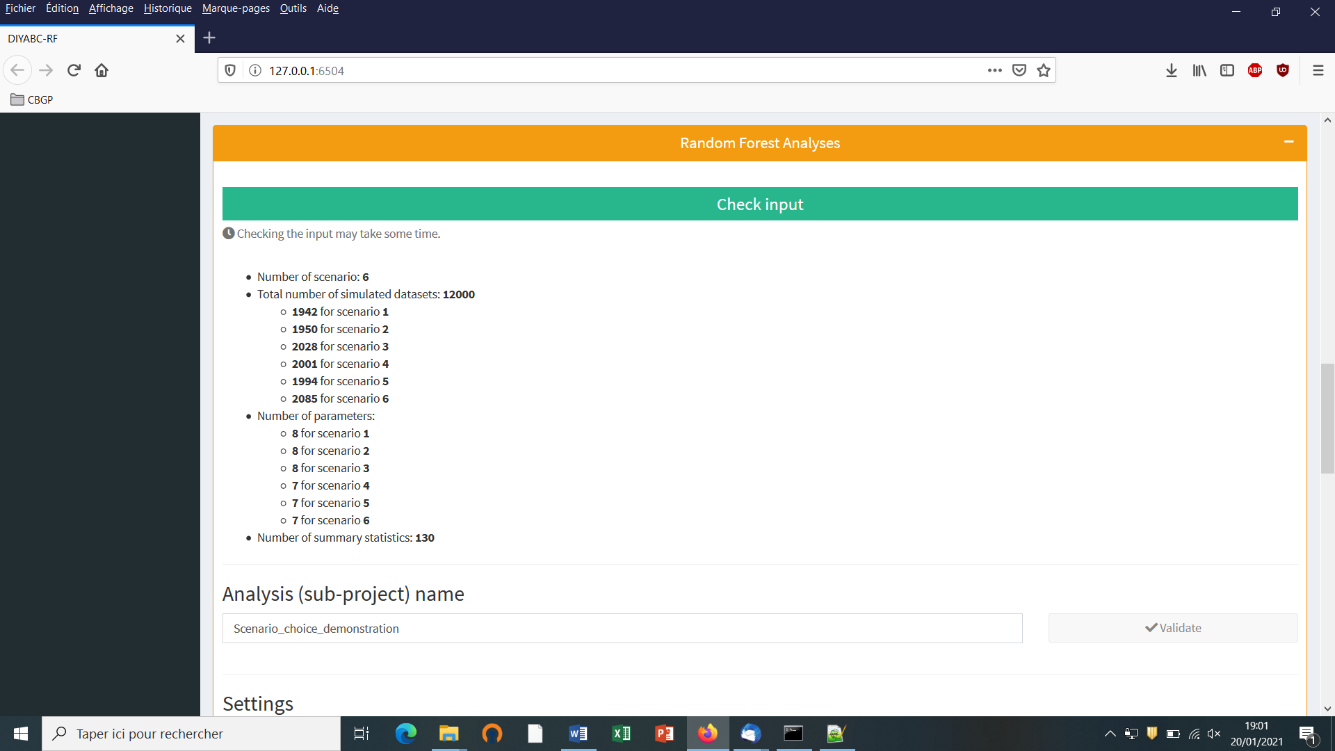
Provide an Analysis (sub-project) name (here “Scenario_choice_demonstration”) and validate it.
Activate the “Scenario choice” button in the mode setting (button activated by default). The observed dataset that will be analyzed is the one described in the file “statobsRF.txt”.

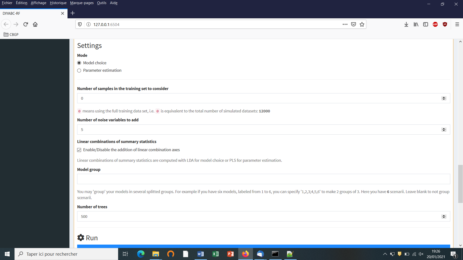
Modify the RF analysis settings in the following frames or keep default settings
Indicate the number of samples (i.e. simulated datasets) in the training set to consider for analyses (default = 0 = total number of simulated datasets available in the training set). This number should be lower or equal to the total number of simulated datasets available in the training set. See section 4.2 for useful insights about this number.
Indicate the number of noise variables to add (default = 5). Noise variables (corresponding to values randomly drawn into uniform distributions bounded between 0 and 1) allows evaluating which components of the feature vector (i.e. summary statistics) are informative (see section 7.3 and Collin et al. 2020 for details).
Enable/disable the addition of linear combinations axes (LDA for model choice) (default = enable)
You may ‘group’ your models in several groups. For instance, if you have six models, labeled from 1 to 6, you can specify ‘1,2,3;4,5,6’ to make 2 groups of 3 scenarios. Leave blank to not group scenarios and analyzed them separately (see Collin et al. 2020). (default = blank). Note that if you write ‘1;3;5’ then the RF scenario choice analysis will concern only the scenarios 1, 3 and 5 of the training set.
Indicate the number of trees in the forest (default = 500). See section 4.3 for useful insights about this number.
Click on the “RUN” button to launch the RF analysis for scenario choice

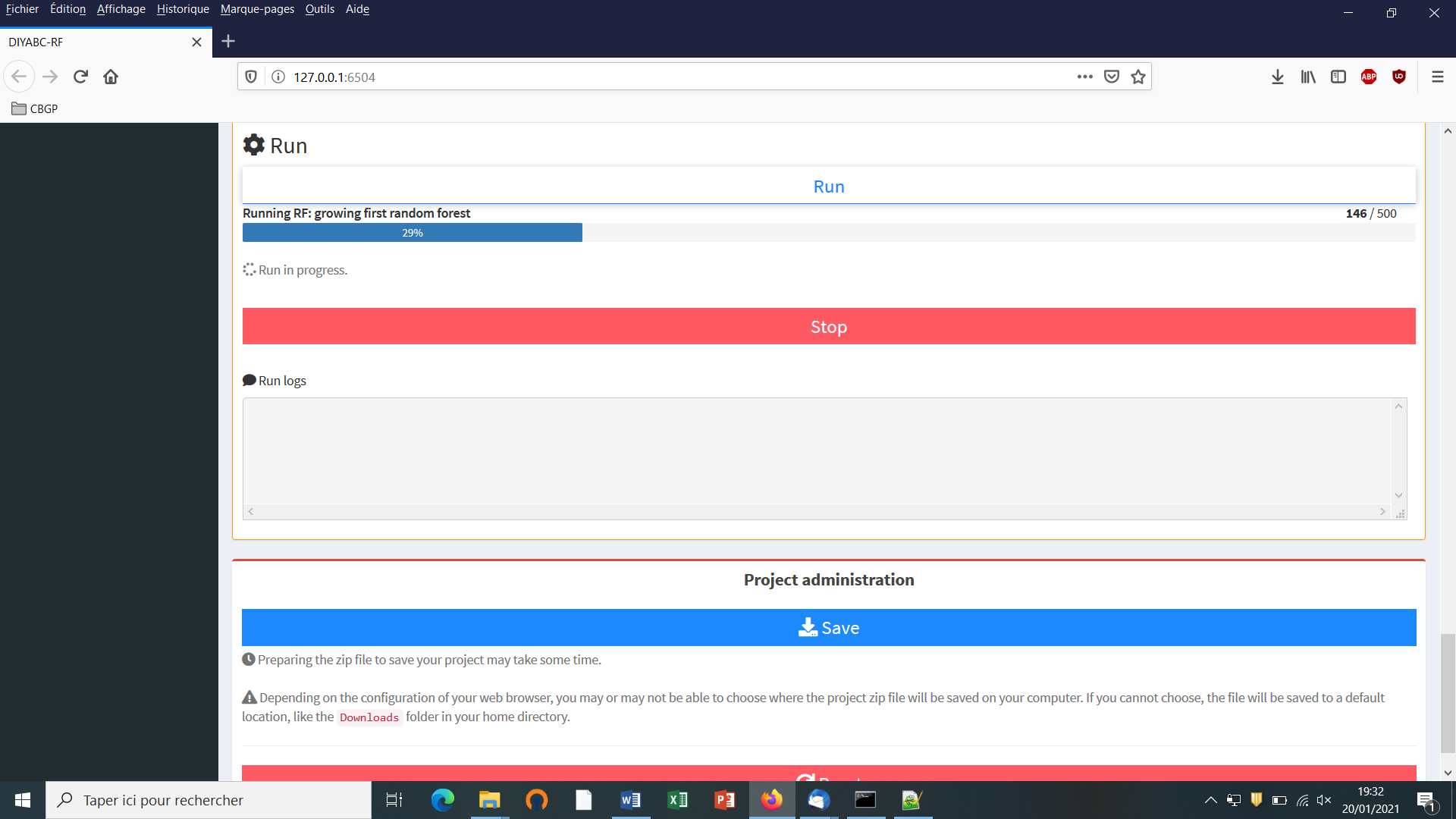
Follow the progress bar. You can stop the RF analysis by clicking on the “STOP” button. A “RF run succeeded” label appears when the RF analysis has been entirely processed.
Do not forget to click on the “Save” button in the “Project administration” panel to implement and save input and output files (see section 7.3 for a description of the content of some of those files) on your computer. These files will be included into a (sub)directory with a name corresponding to the one provided at the start of the model choice analysis (here “Scenario_choice_demonstration”). The corresponding (sub)directory will be itself included within the Project name main directory (here IndSeq_demonstration_project). The ensemble can be loaded as a concatenated zip file (IndSeq_demonstration_project.zip). You can launch and saved several model choice analyses successively by giving different (sub-project) name to each analysis (e.g. “Scenario_choice_demonstration_set1”, “Scenario_choice_demonstration_set2”,…)
Warning: The button “Reset” in the “Project administration” panel restart the pipeline from scratch removing all configurations previously set up and all data and result files generated.

6.3. Parameter estimation analysis

Click on the large orange color “Random Forest Analyses” button (“+” on the right).
Activate the “Parameter estimation” button in the mode setting.
Click on the button “Check input”: Useful information about the training set (cf. reftableRF.bin file) content is provided (nbr of scenarios, total nbr of simulated datasets, nbr of simulated dataset available per scenario, nbr of parameters, nbr of summary statistics).
Provide an Analysis (sub-project) name (here “Parameter_estimation_ra_demonstration”) and validate it.

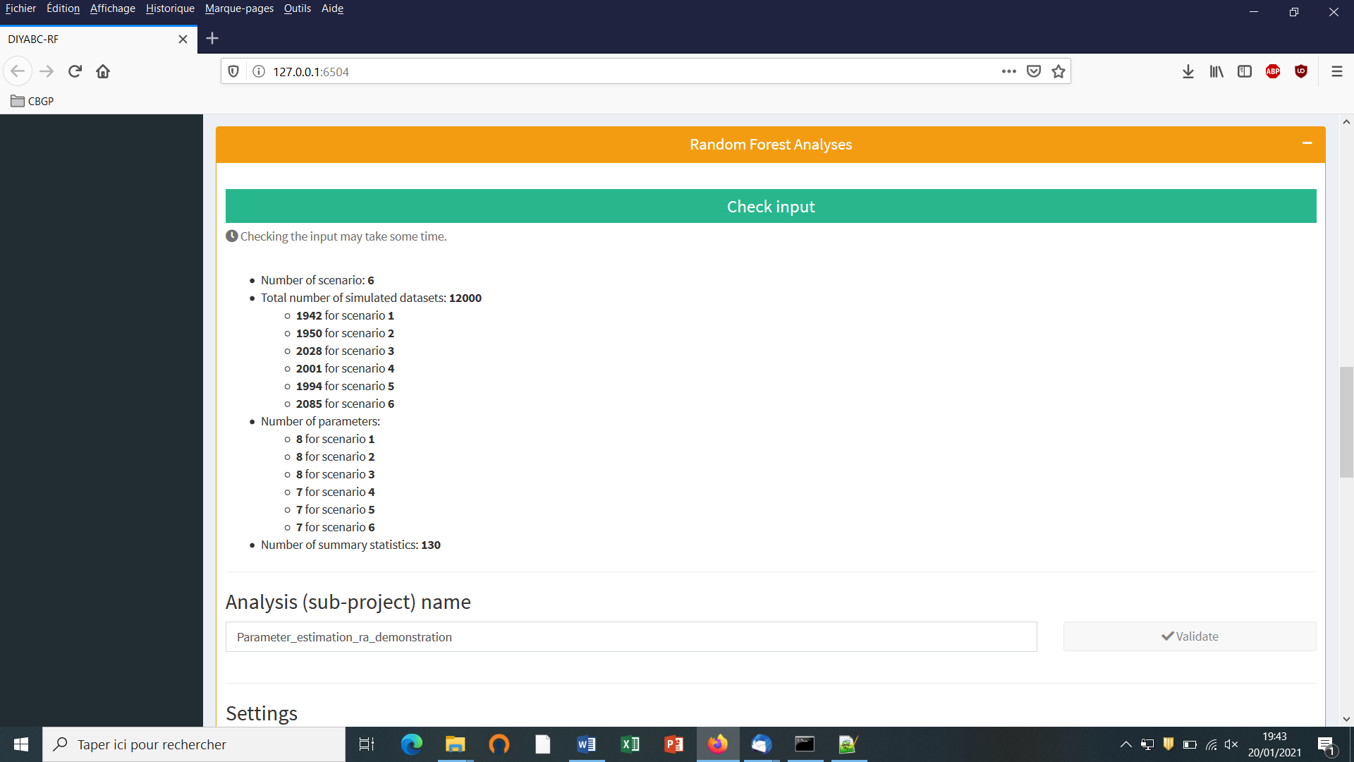
Activate the “Parameter choice” button in the mode setting. The observed dataset that will be analyzed is the one described in the file “statobsRF.txt”.

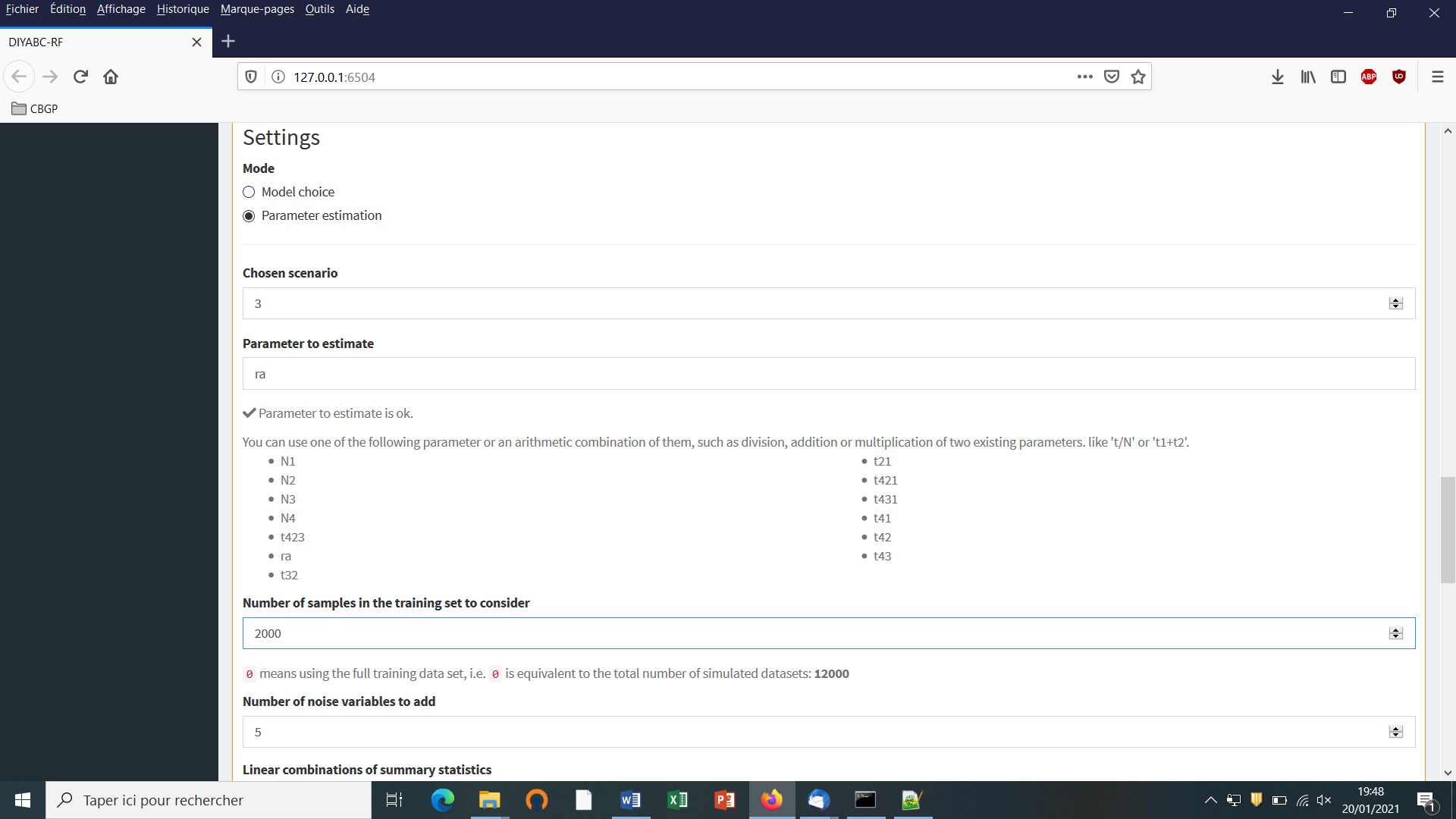
Indicate the ID number of the chosen scenario for parameter estimation (default = 1). Here scenario3.
Indicate the name of the parameter to estimate (here the admixture rate “ra”): a list of parameter names available for estimation according to the header and training set files is provided. Give a single parameter name or a combination of names as explained in the interface. One analysis has to be processed for each parameter of interest.
Indicate the number of simulated datasets in the training set to consider for analyses (default = 0 = total number of simulated datasets available in the training set). Warning: this number should be lower or equal to the total number of simulated datasets available in the training set for the scenario of interest. Here we put this number to 2000 as only 2028 simulated datasets are available for scenario 3 in the reftableRF.bin file previously used for scenario choice and also loaded in the present illustration. See section 4.2 for useful insights about the number of simulated datasets in the training set to consider for parameter estimation. In practice, it might be useful to generate a (second) training set including only the selected scenario to process parameter estimation from a larger number of simulated datasets (e.g. 10000 as in Collin et al. 2020).
Indicate the number of noise variables to add (default = 5). Noise variables (corresponding to values randomly drawn into uniform distributions bounded between 0 and 1) allows evaluating which components of the feature vector (i.e. summary statistics) are informative (see section 7.3 and Collin et al. 2020 for details).

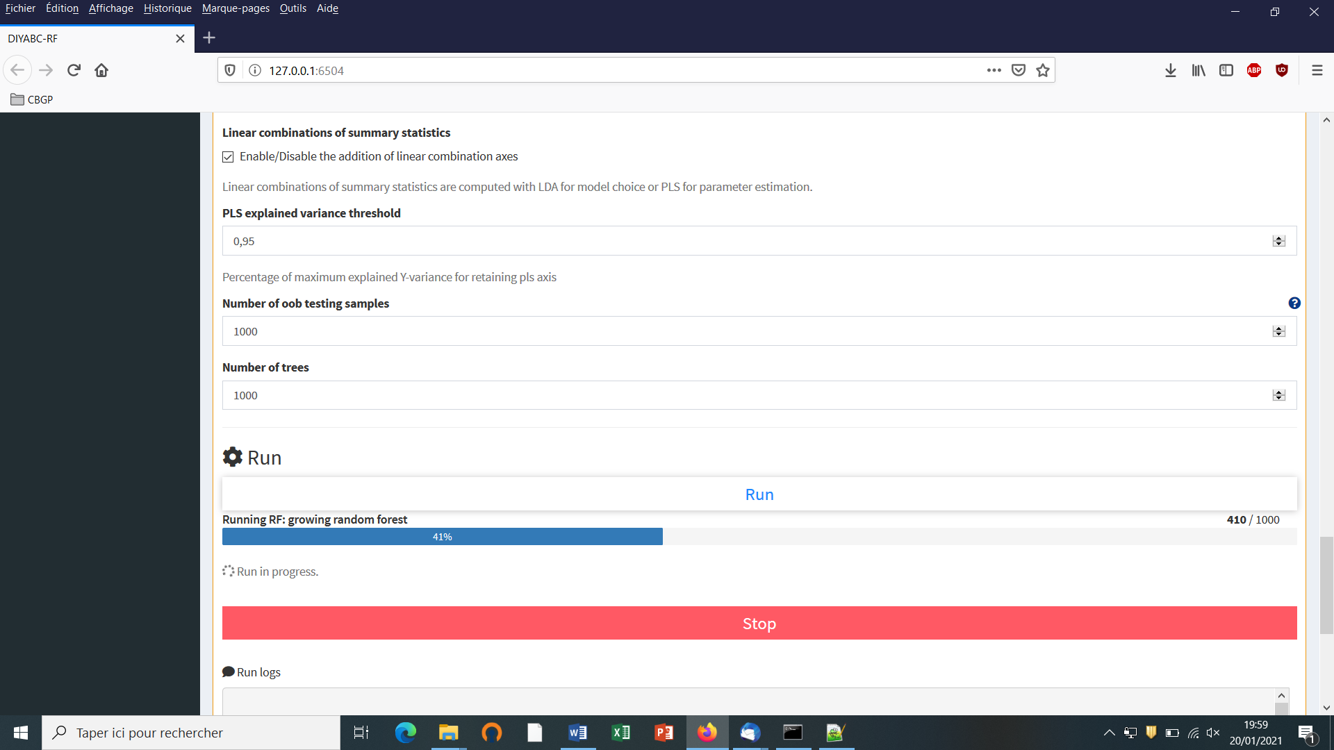
Enable/Disable the addition of linear combinations axes (PLS for parameter estimation) (default = enable)
Indicate the threshold of percentage of explained variance by the PLS components you will keep in the analysis (default = 0.95)
Indicate the number of out-of-bag (oob) testing samples (default = 1000 as a minimum of 1000 oob testing samples is often necessary to obtained stable estimation of accuracy metrics; see section 3.4.2). This number should be equal or lower to the number of datasets available in the training set for the scenario under study.
Indicate the number of trees in the forest – here 1000 - (default = 500). See section 4.3 for useful insights about this number.
Click on the “Run” button to launch the parameter estimation analyses focusing on the single parameter (or parameter combination) indicated above.

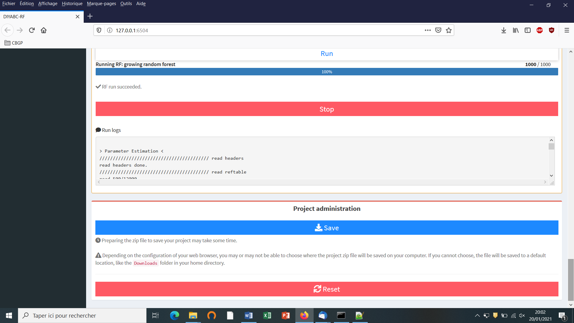
Follow the progress bar. You can stop the RF analysis by clicking on the “STOP” button. A “RF run succeeded” label appears when the RF analysis has been entirely processed.
Do not forget to click on the “Save” button in the “Project administration” panel to implement and save input and output files (see section 7.3 for a description of the content of some of those files) on your computer. These files will be included into a (sub)directory with a name corresponding to the one provided at the start of the model choice analysis (here “Parameter_estimation_ra_demonstration”). The corresponding (sub)directory will be itself included within the Project name main directory (here IndSeq_demonstration_project). The ensemble can be loaded as a concatenated zip file (IndSeq_demonstration_project.zip). You can launch and saved several parameter estimation analyses successively by giving different (sub-project) name to each analysis (e.g. “Parameter_estimation_ra”, “Parameter_estimation_N4”,…)
Warning: The button “Reset” in the “Project administration” panel restart the pipeline from scratch removing all configurations previously set up and all data and result files generated.

7. KEY FILES

The program uses and produces various files that we describe now.

7.1 Data files

7.1.1 IndSeq SNP data

The data file format includes:

A first line (headline) providing the sex-ratio as above (e.g. <NM=1.0NF>, the required MAF (minimum allele frequency criterion; e.g. <MAF=0.05> or <MAF=hudson>), and any text that can be used as a title. The sex ratio of the analyzed species is noted under the form <NM=rNF>, in which r is the ratio of the number of females per male (e.g. <NM=2.5NF> means that the number of males is 2.5 times the number of females; for a balanced sex ratio one should write <NM=1.0NF>). For each SNP, the MAF is computed pooling all genes genotyped over all studied population samples. For instance, the specification of a MAF equal to 5% will automatically select a subset of m loci characterized by a minimum allele frequency ≥ 5% out of the l loci of the observed dataset and only m loci with a MAF ≥ 5% will be retained in a simulated dataset. Writing <MAF=Hudson> (or omitting to write any instruction with respect to the MAF) will bring the program to use the standard Hudson’s algorithm without further selection; see also the above section 2.4.2.
A second line starting with the three keywords IND SEX POP, separated by at least one space, followed by as many letters as SNP loci, the letter giving the location of the locus as above A for autosomal diploid loci, H for autosomal haploid loci, X for X-linked (or haplo-diploid) loci, Y for Y-linked loci and M for mitochondrial loci. Letters are separated by a single space.
As many lines as there are genotyped individuals, with the code-name of the individual, a letter (M or F; or 9 if the sex of the individual is unknown) indicating its sex, and a code-name for its population. **A genotype is defined by the values 0, 1 or 2 which correspond to the number of the (arbitrarily chosen) reference allele composing the genotype** at each SNP locus. For instance, in the case autosomal diploid SNP loci (denoted A), we have: 2 = homozygous genotype for the reference allele (cf. 2 copies of the reference allele), 1 = heterozygous genotype (cf. 1 copy of the reference allele), and 0 = homozygous genotype for the variant allele, with 0 copy of the reference allele. It is worth noting that for autosomal haploid loci (denoted H), as well as for mitochondrial loci (denoted M) and Y-linked loci (denoted Y), the SNP genotypes will be 0 or 1, which is coherent with our logic of defining a genotype according to the number of the reference allele composing the genotype.
Missing SNP genotypes are noted 9 for all type of SNP loci. Missing data are taken into account in the following way. For each appearance of a missing genotype in the observed dataset, the program records the individual and the locus. When simulating datasets, the program replaces the simulated genotype (obtained through the coalescence process algorithm) by the missing data code at all corresponding locations. All summary statistics are thus computed with the same missing data as for the observed dataset. Warning: data files with virtually any amount of missing data can be analyzed by DIYABC-RF. However, for each locus a minimum of one genotyped individual per population is required. This is because summary statistics cannot be computed at a given locus in a given population if only missing data are present.
Only a subset of the SNP loci included in the data file can be considered (selected) in the simulations and hence in subsequent analyses, without modifying the original dataset. For instance, one can choose to select in the corresponding panel the SNP loci 1 to 1000 of a data file including a total of say 10000 loci (see the above section 5.4.4). This allows running faster simulations and processing independent replicate analyses of sets of 1000 SNP loci by considering loci 1 to 1000 and then 1001 to 2000, and so on, in separate analyses.
Following Hudson’s (2002) criterion, only polymorphic SNP loci (over the entire dataset) are considered. Monomorphic SNP loci (over the entire dataset) are automatically filtered by the program. It is preferable, however, that the user removes himself all monomorphic loci from his/her (observed) dataset before submitting it to DIYABC-RF.
Before running any simulation, DIYAB-RF provides a text file including the set of SNP loci selected from the observed dataset (e.g. polymorphic loci 1 to 1000 with a MAF=0.05). This file is named “UserDataFileName.bin.txt”.

EXAMPLE

In our example below, the species is diploid, has an unbalanced sex ratio (i.e. <NM=1.5NF>) and two of its populations were genotyped at 23 SNP loci: 20 autosomal loci, 1 X-linked locus, 1 Y-linked locus and 1 mitochondrial locus. The first line provides the title and includes the species sex-ratio and the MAF (minimum allele frequency). The second line indicates: individual name in column 1, individual sex in column 2 (M for male, F for female, 9 or any other letter if unknown), population name in column 3 and one column per SNP locus (letter A for an autosomal locus, X for an X-linked locus, Y for a Y-linked locus and M for a mitochondrial locus). Columns are separated by one or more spaces. SNP genotypes are coded 0, 1 or 2 (9 for missing data) according to the number of reference alleles at the corresponding locus. In other words, the homozygous genotype 2 has two reference alleles, the homozygous genotype 0 has two non-reference alleles and the heterozygous genotype 1 has one reference allele and one non-reference allele. Note that the sex has no influence on simulations for autosomal, mitochondrial or haploid loci (any sex can be hence declared). For individuals with an unknown sex (denoted 9, see IND P1_2, P1_3 and P2_15), data for autosomal (as well as mitochondrial and haploid) loci will be taken into account and simulated. On the other hand, the genotypes of X-linked and Y-linked loci for the same IND P1_2, P1_3 and P2_15 with unknown sex cannot be safely determined and are hence noted 9 for missing data (i.e. they are not simulated).

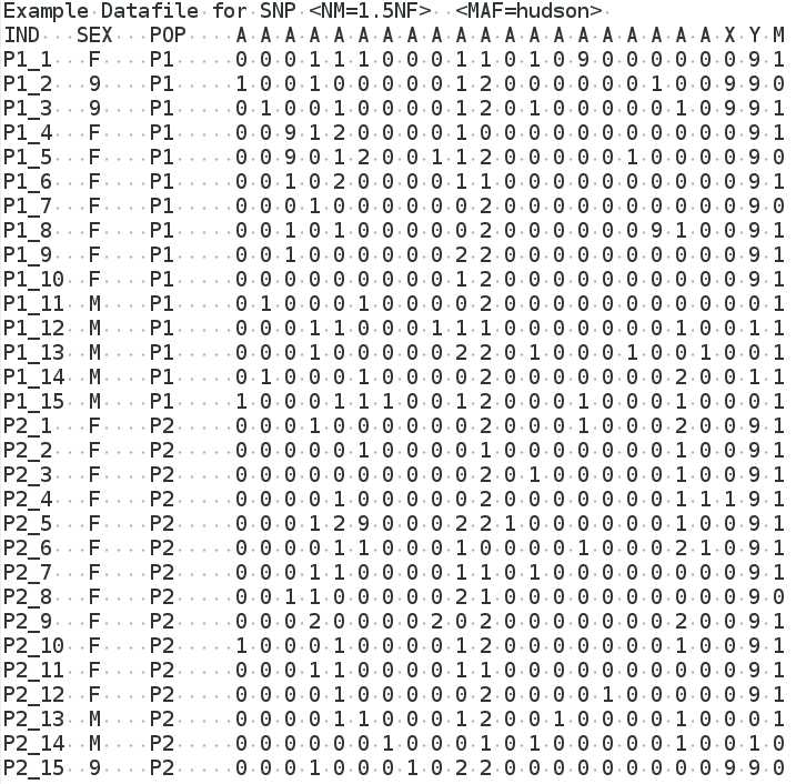
7.1.2 PoolSeq SNP data

The data file format includes:

A first line (headline) providing the sex-ratio of the analyzed species (e.g. <NM=1.0NF>), the required MRC (minimum read count criterion; e.g. <MRC=5>), and any text that can be used as a title. The sex ratio is noted under the form <NM=rNF>, in which r is the ratio of the number of females per male (e.g. <NM=2.5NF> means that the number of males is 2.5 times the number of females; for a balanced sex ratio one should write <NM=1.0NF>). The MRC is the minimum number of sequence reads for each alleles of a SNP when pooling the reads overall population samples. The specification of a MRC equal to 5 will automatically select a subset of m PoolSeq loci for which both alleles have at least five reads among the l loci of the observed dataset. For instance, the first locus of the list (cf. third line of the file) will not be selected. In agreement with this, and only m loci with a MRC ≥ 5 will be retained in a simulated dataset. We advise using MRC values of 2, 3, 4 or 5.
Remember that (in contrast to IndSeq SNP) only PoolSeq SNPs located on autosomal chromosomes of diploid individuals can be considered by the program.
A second line provides the haploid sample size of each population pool.
The following lines correspond to the PoolSeq SNP genotypes (given in read counts). Each line represents a SNP and each pair of columns points to a population pool in the same order as in the second line. For each SNP-pool combination, the number of read counts is indicated for the first and second allele in the first and second column, respectively.
Warning: no missing data (i.e. “0 0” data; cf. no read count for any allele) is allowed in the PoolSeq data file and this for any pools in the data file.
We advise to put only SNP loci with a coverage > 10 reads for each analyzed pool of the dataset in order to ensure descent allele frequency estimation within each pool. SNP loci with an abnormally high coverage should be also removed as those loci can be duplicated loci.
Only a subset of the SNP loci included in the data file can be considered (selected) in the simulations and hence in subsequent analyses, without modifying the original dataset. For instance, one can choose to select in the corresponding panel the SNP loci 1 to 1000 of a data file including a total of say 10000 loci (see the above section 5.4.4). This allows running faster simulations and processing independent replicate analyses of sets of 1000 SNP loci by considering loci 1 to 1000 and then 1001 to 2000, and so on, in separate analyses.

EXAMPLE

In our example below, the species is diploid and was genotyped using the PoolSeq technology at several thousands of autosomal SNPs in four population pools; only the first 13 SNPs are shown here for sake of concision. The species sex-ratio is balanced and hence equal 1 and the MRC (minimum read count) is 5. Each population pool is composed of 100 diploid individuals (haploid sample size = 200). The second line provides the haploid sample size of each population pool. It has to start with the explicit terminology POOL POP_NAME:HAPLOID_SAMPLE_SIZE. Here the haploid sample size is 200 for each “POPx”. Note that you can write any sample name, e.g. MONTPELLIER, instead of POPx. Columns are separated by one or more spaces. Each line represents a SNP (hence the 13 lines) and each pair of columns points to a population pool (hence the 4 pairs of column). For each SNP-pool combination, the number of read counts is indicated for the first and second allele in the first and second column, respectively. For instance, we have 2 reads of the first allele and 114 reads of the second allele for the first SNP genotyped in the POOL-POP3. Note that because the MRC=5 several SNP of the present example data file, e.g. the first SNP for which only two read counts are present over all pools, will not be selected when generating simulated datasets.

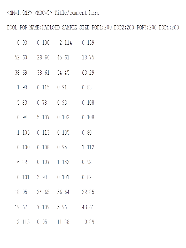
7.3.1 Microsatellite and DNA sequence data

The data file format is an extended format of the file used in the classical population genetics program Genepop (Rousset et al. 1995). The additional features are:

In the title line appears the sex ratio noted <NM=rNF>, in which $r$ is the ratio of the number of females per male (e.g. NM=2.5NF) means that the number of males is 2.5 times the number of females; for a balanced sex ratio one should write<NM=1.0NF>. Since the title is generally only copied, this addition should not interfere with other programs using Genepop datafiles. Also if there is no such sex ratio addition, DIYABC-RF will consider by default that NM=1.0NF.
After the locus name, there is an indication for the category of the locus which is A for autosomal diploid loci <H> for autosomal haploid loci, <X> for X-linked (or haplo-diploid) loci, Y for Y-linked loci and <M> for mitochondrial loci. If no category is noted, DIYABC-RF will consider the locus as autosomal diploid or autosomal haploid depending on the corresponding genotype of the first typed individual.
Genotypes of microsatellite loci are noted with six digit numbers if diploid (e.g. 190188 for a heterozygous genotype with one allele 190 and one allele 188, and 200200 for a homozygous genotype with two alleles 200) and by three digit numbers (e.g. 190) if haploid. The three digit numbers correspond to the length in nucleotides of the corresponding PCR products.
Sequence locus are noted between < and >. In addition, each sequence alleles/haplotypes is noted between brackets. For instance, a haploid sequence locus will be noted <[GTCTA]> and a diploid sequence locus <[GTCTA][GTCTT]>. Sequences may contain undetermined nucleotides which will be denoted “N “ or “ - “. Note that all sequence alleles/haplotypes have to be of same length. The length of shorter sequence allele/haplotypes needs to be adjusted to the larger sequence allele/haplotype by adding “N “ or “ - “ symbols at the end of the sequences. It is worth stressing that, at a given locus, only the portion of the sequence shared by all individuals of the dataset will be used for computing summary statistics. We therefore advise removing locus-individual sequence data with too many “N” and replace them by missing data. Finally, remember that this version of the program does not consider insertion-deletion mutations, mainly because there does not seem to be much consensus on this topic.
Missing microsatellite genotypes are noted 000 if haploid or 000000 if diploid.
Missing sequence alleles/haplotypes are noted <[ ]> if haploid or <[ ][ ]> if diploid.
Missing data are taken into account in the following way. For each appearance of a missing genotype in the observed dataset, the program records the individual and the locus. When simulating datasets, the program replaces the simulated genotype (obtained through the coalescence process algorithm) by the missing data code at all corresponding locations. All summary statistics are thus computed with the same missing data as for the observed dataset. Warning: data files with virtually any amount of missing data can be analyzed by DIYABC-RF. However, for each locus a minimum of one genotyped individual per population is required. This is because summary statistics cannot be computed at a given locus in a given population if only missing data are present.

EXAMPLES

Example 1: the example dataset below includes two population samples, each of 12 diploid individuals (8 females and 4 males in the first sample and 5 females and 7 males in the second sample). As deduced from the letter between and on the locus name lines (see page 25), these individuals have been genotyped at 3 microsatellite loci (1 autosomal <A>, 1 X-linked <X> and 1 Y-linked <Y>) and 3 DNA sequence loci (1 autosomal <A>. 1 X-linked <<X> and 1 mitochondrial <M>). The species sex-ratio, given in the title line, is of three males for one female (<NM=3NF>) or in other words, the number of males equals three times the number of females.

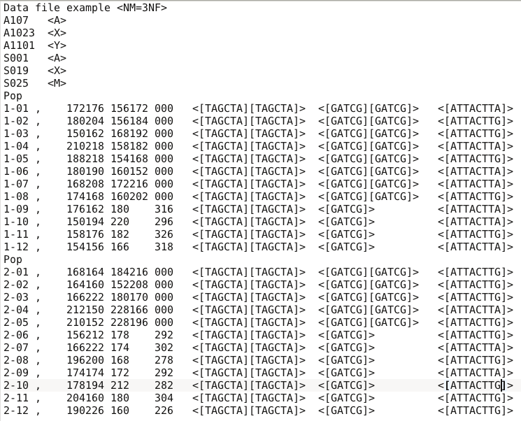
Example 2: in this second example, the species is haploid. Individuals have been genotyped at three autosomal microsatellite loci and one mitochondrial DNA sequence locus. The species being haploid (deduced from the presence of autosomal haploid loci), no indication of the sex-ratio appears in the title line.

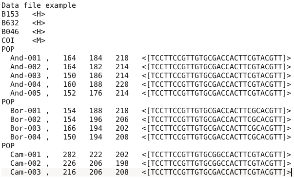
7.2 Training set file(s)

Training set files are binary files which include two successive parts:

The first file is a header (named headerRF.txt) which contains information necessary to read the second part (file), such as the number of scenarios, or the number of parameters of each scenario.
The second file (named reftableRF.bin) corresponds to the training set per se, as this file contains simulated dataset records, each record containing on the same line the scenario number, the parameter values and summary statistics values.

Each time a training set (reftableRF.bin) is created or increased (each time the training set “Run” button is pressed), two text files are created in the project directory:

statobsRF.txt: this text file contains the values of summary statistics for the observed data set.
first_records_of_the_reference_table_X.txt in which X is an integer number starting at 0 and increasing each time the training set “Run” button is pressed. This file provides a text version of the first $n$ newly created records of the training set reftableRF.bin ($n$ being equal to the Particle loop size, see section 3.7.3).

7.3 Output files produced by a Random Forest analysis

DIYABC-RF provides various numerical and graphical outputs. The integration of the various graphical outputs is managed with the ggplot2 R package (Wickham 2016), allowing user to create and export high-quality graphics related to the analyses. Non-graphical outputs are saved in text files. Graphs are saved as images, and user can choose the image format among png, jpg, etc.

We now describe all the files produced by each Random Forest analysis.

abcranger_call.log: log files with votes and posterior probability of the selected (i.e. best) scenario (i.e. model) for a model choice analysis and with the main outputs of parameter estimation (including predictions and accuracy of estimation metrics) for a parameter estimation analysis.

Scenario choice analysis

Numerical outputs

modelchoice_out.settings: this file summarizes the settings associated to the RF analysis processed for scenario choice.

modelchoice_out.confusion: mean misclassification error rate (also named global prior error rate; Collin et al. 2021) and confusion matrix (i.e. the contingency table of the true and predicted classes for each example in the training set). These metrics are computed using the out-of-bag (a.k.a. out-of-bootstrap or oob) training data as free test dataset.

modelchoice_out.predictions: votes, prediction of the selected scenario and posterior probability of the selected scenario (i.e. model).

modelchoice_out.ooberror: Evolution of prediction power relatively to the number of trees in the forest. Line number is the number of trees. Power is the global (prior) error rate for scenario choice (computed using oob). See the file modelchoice_out_graph_error_versus_ntrees.png for a graphical representation.

modelchoice_out.importance: variables importance (sorted) which correspond to the contributions of the statistics to the Random Forest when choosing among scenarios. The variable importance of each statistics is computed as the mean decrease of impurity across the trees, where the impurity measure is the Gini index. Note that the scale is irrelevant: only the relative values matter. The variable importance was computed for each of the summary statistics provided by DIYABC-RFt, plus the LDA axes (denoted LDA) if they have been added to the feature vector. The higher the variable importance the more informative is the statistic. Variable importance of noise variables (denoted NOISEx and corresponding to values randomly drawn into uniform distributions bounded between 0 and 1) are also provided. Such noise variable can be added to the feature vector processed by RF in order to evaluate the threshold of variable importance values below which components of the vector are not informative anymore. More details about summary statistics including their code names can be found in section 2.6.3. Population index(s) are also indicated at the end of each statistic. See Collin et al. 2020 for examples. See the file modelchoice_out_graph_variable_importance.png for a graphical representation.

modelchoice_out.lda: coordinates for the projection of the datasets from the training set and from the observed dataset on the first two linear discriminant analysis (LDA) axes when analyzing more than two scenarios (models) and on a single LDA axis when analyzing a pair of scenarios (or two groups of scenarios); See the file modelchoice_out_graph_lda.png for a graphical representation.

Graphical outputs

modelchoice_out_graph_lda.png: Projection of the datasets from the training set on the first two linear discriminant analysis (LDA) axes when analyzing more than two scenarios (models) and on a single LDA axis when analyzing a pair of scenarios (or two groups of scenarios). The location of the observed dataset in the LDA projection is indicated by a specific symbol or a vertical line. Such Graphical representation has been obtained from the text file modelchoice_out.lda; see also Figure 2 in Collin et al. 2020.

modelchoice_out_graph_error_versus_ntrees.png: Evolution of prediction power relatively to the number of trees in the forest. Such graphical representation has been obtained from the text file modelchoice_out.ooberror ; see also Figure S1 in Collin et al. 2020.

modelchoice_out_graph_variable_importance.png: Contributions of the 50 most informative statistics (including LDA axes if computed) to the Random Forest when choosing among scenarios. Such graphical representation has been obtained from the text file modelchoice_out.importance; see also Figure 3 in Collin et al. 2020.

Parameter estimation analysis

Numerical outputs

estim_param_out.settings: this file summarizes the settings associated to the RF analysis processed to estimate a given parameter

estim_param_out.predictions: expectation, median, quantiles 0.05, quantile 0.95, and variance for prediction of parameter estimation

estim_param_out.ooberror: Evolution of prediction power relatively to the number of trees in the forest. Line number is the number of trees. Power is the global (prior) mean squared error with the mean taken as point estimate (computed using oob). See the file estim_param_out_graph_error_versus_ntrees.png for a graphical representation.

estim_param_out.oobstats: this file contains various accuracy metrics of parameter estimation (computed using oob). Both global (prior) error metrics and Local (posterior) error metrics are provided; See section 3.4.2 Metrics for parameter estimation and Collin et al. 2020 for details).

estim_param_out.importance: variables importance (sorted) which correspond to the contributions of the statistics to the Random Forest when processing parameter estimation. The variable importance of each statistics is computed as the mean decrease of impurity across the trees, where the impurity measure is the residual sum of squares. Note that the scale is irrelevant: only the relative values matter. The variable importance was computed for each of the summary statistics provided by DIYABC-RF, plus the PLS axes (denoted Comp.) if they have been added to the feature vector. The higher the variable importance the more informative is the statistic. Variable importance of noise variables (denoted NOISEx and corresponding to values randomly drawn into uniform distributions bounded between 0 and 1) are also provided. Such noise variable can be added to the feature vector processed by RF in order to evaluate the threshold of variable importance values below which components of the vector are not informative anymore. More details about summary statistics including their code names can be found in section 2.6.3. Population index(s) is also indicated at the end of each statistic. See Collin et al. 2020 for examples. See the file estim_param_out_graph_variable_importance.png for a graphical representation.

estim_param_out.predweights: pairs of parameter value - weight value inferred during prediction. Such pairwise values can be used to do density plot of parameter estimation. See the file estim_param_out_graph_density_plot.png for a graphical representation.

If a Partial Least Squares Regression analysis (PLS) is processed on the summary statistics then two additional output files are provided.

estim_param_out.plsvar: variance explained by number of the c selected PLS components (from component 1 to c, with c the number of PLS axes providing a given fraction of the maximum amount of variance explained by all PLS axes - 95% by default-).

estim_param_out.plsweights: weight of each variable (i.e. summary statistics) for the first PLS component (sorted by absolute value)

Graphical outputs

estim_param_out_graph_density_plot.png: density plot graphical representation for the estimated parameter (obtained from the text file estim_param_out.predweights).

estim_param_out_graph_error_versus_ntrees.png: Evolution of prediction power relatively to the number of trees in the forest. Such graphical representation has been obtained from the text file estim_param_out.ooberror; see also Figure S1 in Collin et al. 2020.

estim_param_out_graph_variable_importance.png: Contributions of the 50 most informative statistics (including PLS components – denoted as Comp - if computed) to the Random Forest when choosing among scenarios. Such graphical representation has been obtained from the text file estim_param_out.ooberror; see also Figure 3 in Collin et al. 2020.

7.4 Other files

The program writes several additional files in the saved project directory:

diyabc_run_call.log: this text file contains information about the first steps of the training set production, including the reading of the observed data file and the interpretation of the headerRF.txt file.

reftable.log: this file contains information about the progress of computations (achieved number of records)
RNG_state_0000.bin: this binary file contains the current state of the random generator.

diyabc_seed_init_call.log: this text file contains information about the initialization of the random generator

Files produced with IndSeq analysis

<observed_dataset_name>.bin and <observed_dataset_name>.txt: observed dataset file in bin and txt format, respectively
maf.txt: file in which the minimum allele frequency value (maf) has been recorded

8. GENERATE SYNTHETIC DATAFILES

An (auxiliary) module named “Synthetic data file generation” (based on the DIYABC-RF simulation engine) is available in the package. You can use this module to generate datafile(s) for various types of genetic markers corresponding to synthetic “ground truth” raw data (i.e. not summarized through statistics) under a given historical scenario and a set of parameter values fixed by the user. Such pseudo-observed dataset does not refer to any (actual) observed dataset. The formats of the generated datafiles are similar to those of the observed input datafiles read by DIYAB-RF (see sections 7.1.1, 7.1.2 and 7.1.3).

To access to the panels allowing generating files corresponding to full in silico datasets (also called pseudo-observed datasets) click on the “Synthetic data file generation” button in the middle of the main panel of the GUI or on the “Synthetic data file generation” button in the upper-left part of the same panel.

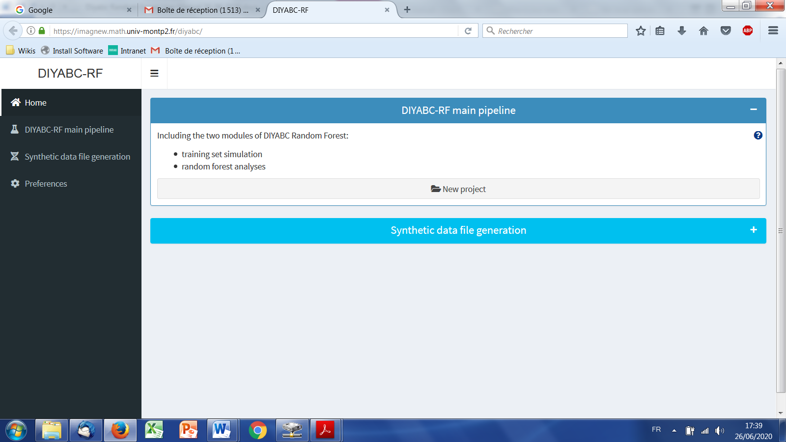
The panels following such clicking are very similar to those detailed in the sections 5.4 (IndSeq data), 5.5 (PoolSeq data) and 5.6 (microsatellite and/or DNA sequence data) and are thus not shown here. Their self-meaning content allows defining a scenario, fixing prior values for historical (and genetic) parameters, and the number (and type) of loci to simulate. It is worth stressing that those panels are completed by two (also self-meaning) additional panels in which you indicate the sample sizes for each population (with the proportion of males and females in each sample), the sex ratio of the studied species, and the number of datafiles that you want to simulate. For the simulation of pseudo-observed PoolSeq datasets the user is asked for a read coverage value (default value: coverage = 100X).

9. USING DIYABC-RF ON A COMPUTER SERVER AND EXAMPLES OF COMMAND LINES

The computing effort is considerably reduced for ABC Random Forest, as the method requires a substantially smaller training set compared to traditional ABC methods (e.g., a few thousands of simulated datasets versus hundreds of thousands of simulations per scenario for most ABC approaches; Blum & François, 2010; Fraimout et al., 2017; Pudlo et al., 2016; Raynal et al., 2019). Given the ever-increasing dimensionality of modern genetic data generated using NGS technologies, this is a particularly appealing property of this method. Your personal computer or any local server should hence represent sufficient computer resources to run most of your DIYABC-RF analyses in a descent time. However, in some cases (for instance when very large SNP datasets have to be simulated), it might be useful to take advantage of a compute server (single node of a cluster, or even a powerful workstation), especially to generate the training set (i.e. the file reftableRF.bin).

To do this (i.e. generate the reftableRF.bin training set), go to the DIYABC-RF main site https://diyabc.github.io/ at the Command line tools section to find the diyabc v3.0 binary (executable) file corresponding to your Operating System. Compilation and command line instructions are also available at the github repository for diyabc RF.

Similarly, compilation, command line instructions as well as the sources and various binary versions of the program abcranger, which is the Random Forest inference engine of the program DIYABC-RF, are also available at the github repository for abcranger. However, this might be less crucial as Random Forest treatments with abcranger (using a given training set) are much more rapid than the generation of the training set with diyabc v3.0 (e.g. Collin et al. 2020).

EXAMPLES OF COMMAND LINES

Warning: for additional details and options see instructions in Commande line tools - DIYABC RF

Simulation of a training set using the (linux) executable file diyabc_vXXX (where XXX is the version)

Put in a given directory the following files:

The file corresponding to your (observed) dataset
The header file which can be the headerRF.txt file or a header.txt file, the later file corresponding to the standard header file of DIYABC v2.1.0 (Cornuet et al. 2014) in which any number and type of summary statistics is specified. This allowed users to “recycle” header files that they might have previously produced with DIYABC v2.1.0. It is worth stressing that the program rewrites and produces automatically - using the headerRF.txt file or the header.txt file as starting point - a headerRF.txt file with all necessary information and including all available summary statistics for RF analysis to feed diyabc_vXXX and start simulation of the training set. Note that the standalone DIYABC–RF too can cope with a standard header file (i.e. header.txt) of DIYABC v2.1.0.
The file RNG_state_0000.bin, which you should generate at first in a terminal window with:

./diyabc_vXXX -p ./ -n “t:8”

where you can replace 8 by the number of computing cores of your server.

You can then launch the simulation in a terminal window with:

./diyabc_vXXX -p ./ -R ALL -r 12000 -g 50 -m -t 8

By doing so you will simulate a training set (reftableRF.bin) including 12000 datasets with all summary statistics available in DIYABC-RF (plus LDA axes added to the feature vector) and using a loop size of 50 simulated datasets and a total of 8 cores (you can specify at most the number of cores specified by the previously generated RNG_state_***.bin file) .

Random Forest analyses using the (linux) executable file abcranger_vXXX

Put in a given directory the following files:

The file headerRF.txt (previously generated by diyabc_vXXX)
The file reftableRF.bin (previously generated by diyabc_vXXX) corresponding to the training set
The file statobsRF.txt (previously generated by diyabc_vXXX) which contains the values of summary statistics for the observed data set.

Model (scenario) choice using RF

You can then launch the analysis in a terminal window with:

./abcranger_vXXX -n 12000 -t 1000 -j 8 -o modelchoice_analysis

By doing so you will process a model choice analysis on 12000 datasets of the training set with a forest including 1000 trees, with error metrics computed from 12000 out-of-bag (oob) datasets, and using a total of 8 cores. All output files names will have “modelchoice_analysis” as prefix.

Parameter estimation (t) using RF

You can launch the analysis in a terminal window with:

./abcranger_vXXX -n 2000 -t 1000 -j 8 –parameter t –chosenscen 1 –plsmaxvar 0.95 –noob 10000 -o estim_param_t_with_PLS

By doing so you will process an estimation of the parameter t from 2000 datasets (if available in the training set) with a forest including 1000 trees, with a number of PLS components explaining 95% of variance added to the feature vector, with accuracy metrics computed from 10000 out-of-bag (oob) datasets, and using a total of 8 cores. All output files names will have “estim_param_t_with_PLS” as prefix.

Note: The pipeline and command lines used to generate and analyze the example datasets in Collin et al. (2020) can be consulted at https://github.com/diyabc/MER\_publication\_materials/tree/main/MER\_2021\_DATASET\_EXAMPLES

It is worth stressing that abcranger is not limited to population genetics applications as you can use the program as a Random Forest inference engine independently from the diyabc simulator. However, for the moment, the binary standalone used by the DIYABC-RF interface handles only outputs produced by the DIYABC-RF simulator. A python wrapper (and example notebooks) is available at the notebook directory in the github repository and a R wrapper will be soon provided at the same site.

10. TOY EXAMPLES

Five toy examples to process run-tests with DIYABC-RF (i.e. for a quick generation of a training set and rapid Random Forest analyses) can be downloaded from https://diyabc.github.io/toy_examples/. Each toy example illustrates crucial aspects such as the formats of different types of observed datasets, the formalization of different types of scenarios and the using of various types of molecular markers. Each toy example includes two files: an observed dataset file and a “ready to use” headerRF.txt file. You can launch directly the ABC-RF standalone by choosing the “Existing project” option and loading these two files.

TOY_EXAMPLE1_microsatellites_one_pop_bottlenecked

The pseudo-observed dataset includes a single population bottlenecked at time tbn in the past with 4 samples (20 individuals per sample) taken at different times. Note that NM=1.0NF, Npresent= 200, tbn=300, Npass=20000. The dataset includes 45 autosomal microsatellite loci and 5 mitochondrial microsatellite loci with 2 groups of mutation parameters.

The headerRF.txt file formalizes two scenarios: one with and one without a bottleneck event.

TOY_EXAMPLE2_microsatellites_DNAsequence_two_pops_ancient_admixture

The pseudo-observed dataset includes two populations with ancestral admixture between two unsampled pops at time ta=5000 (ra=0.5) that diverged at time t2=6000 with N1=5000 and t1=1000 for 10 autosomal microsatellites 5 autosomal DNA sequences and 5 mitochondrial DNA sequences with 3 groups of mutation parameters.

The headerRF.txt file formalizes two scenarios: one with and one without an ancestral admixture event.

TOY_EXAMPLE3_SNP_INDSEQ_scenario3_MER_light_configuration

This toy example is similar to the IndSeq SNP illustration of the paper Collin et al. (2020) based on the pseudo-observed dataset generated from scenario 3, except that only 100 SNP (instead of 5000) are requested for simulation in the headerRF.txt file formalizing 6 scenarios to speed-up simulations.

Warning: because only 100 SNP are simulated, do not expect to obtain the same results as those described in Collin et al. (2020).

TOY_EXAMPLE4_SNP_POOLSEQ_scenario3_MER_light_configuration

This toy example is similar to the PoolSeq SNP illustration of the paper Collin et al. (2020) based on the pseudo-observed dataset generated from scenario 3, except that only 100 SNP (instead of 5000) are requested for simulation in the headerRF.txt file formalizing 6 scenarios to speed-up simulations.

Warning: because only 100 SNP are simulated, do not expect to obtain the same results as those described in Collin et al. (2020).

TOY_EXAMPLE5_SNP_INDSEQ_several_groups_of_loci_admixture

The IndSeq SNP pseudo-observed dataset includes three populations with pop 3 admixed between pops 1 and 2 at time ta=100 (r=0.4) and pops 1 and 2 diverging at time ts=10000 (N1=20000, N2=5000, N3=10000, N4=10000). Note that NM=0.428571NF and MAF=Hudson. The dataset includes SNP loci of different types: A=700 loci, X=100, Y=100 and M=100.

The headerRF.txt file formalizes three scenarios: one with and two without admixture event. The headerRF.txt file requests only A=70 loci, X=10, Y=10 and M=10 to speed-up simulations.

11. REFERENCES CITED

Beaumont M. 2010. Approximate Bayesian computation in evolution and ecology. Annual Review of Ecology, Evolution, and Systematics, 41, 379–406.

Breiman, L., 2001. Random forests. Machine Learning, 45(1), 5–32.

Blum MGB, François O. 2010.Non-linear regression models for Approximate Bayesian Computation. Statistics and computing. 20(1):63–73. https://doi.10.1007/s11222-009-9116-0

Chang W, Cheng J, Allaire JJ, Xie Y, McPherson J ,2019. Shiny: Web Application Framework for R. R package version 1.4.0. https://CRAN.R-project.org/package=shiny

Chapuis M-P, R. Raynal, L, Plantamp, C, Meynard, CN, Blondin, L. Marin J-M, Estoup A. 2020. A young age of subspecific divergence in the desert locust Schistocerca gregaria, inferred by ABC Random Forest. Molecular Ecology 29(23), 4542-4558. https//doi:10.1111/mec.15663. Previous version reviewed and recommended by Peer Community in Evolutionary Biology, bioRxiv, 671867, 10.24072/pci.evolbiol.100091

Choisy M, P. Franck, Cornuet J-M. 2004. Estimating admixture proportions with microsatellites: comparison of methods based on simulated data. Molecular. Ecology 13, 955-968.

Chakraborty R, L Jin, 1993. A unified approach to study hypervariable polymorphisms: statistical considerations of determining relatedness and population distances. EXS. 67, 153?175.

Collin F-D, Raynal L, Durif G, Gautier M, Vitalis R, Marin J-M, Estoup A. 2020. DIYABC Random Forest v1.0: extending approximate Bayesian computation with supervised machine learning to infer demographic history from genetic polymorphisms. Molecular Ecology Resources. https://doi: 10.22541/au.159480722.26357192

Cornuet J.M, Ravigné V, Estoup A. 2010. Inference on population history and model checking using DNA sequence and microsatellite data with the sofware DIYABC (v1.0). BMC Bioinformatics 11,401.

Cornuet J.M., F. Santos, M.A. Beaumont, C.P. Robert, J.M. Marin, D.J. Balding, T. Guillemaud, Estoup A. 2008. Infering population history with DIYABC: a user-friendly approach to Approximate Bayesian Computations. Bioinformatics, 24 (23), 2713-2719.

Cornuet J-M, Pudlo P, Veyssier J, Dehne-Garcia A, Gautier M, Leblois R, Marin J-M, Estoup A. 2014. DIYABC v2.0: a software to make approximate Bayesian computation inferences about population history using single nucleotide polymorphism, DNA sequence and microsatellite data. Bioinformatics. Vol. 30, no. 8, p11871189, doi: 10.1093/bioinformatics/btt763.

Jarne P, Cornuet J-M. 2002. Homoplasy and mutation model at microsatellite loci and their consequences for population genetics analysis. Molecular Ecology., 11, 1591-1604.

Estoup A, Raynal L, Verdu P, Marin J-M. 2018. Model choice using Approximate Bayesian Computation and Random Forests: analyzes based on model grouping to make inferences about the genetic history of Pygmy human populations. Journal de la Société Française de Statistiques, 159(3), 167-190.

Excoffier L, Estoup A, Cornuet J-M. 2005. Bayesian analysis of an admixture model with mutations and arbitrarily linked markers. Genetics 169, 1727-1738.

Fraimout A, Debat V, Fellous S, Hufbauer RA, Foucaud J, Pudlo P, Estoup A. 2017. Deciphering the routes of invasion of Drosophila suzukii by means of ABC Random Forest. Molecular biology and evolution, 34(4), 980–996. https:// doi.10.1093/molbev/msx050

Garza JC, Williamson E. 2001. Detection of reduction in population size using data from microsatellite DNA. Molecular Ecology 10,305-318.

Gautier M, Foucaud J, Gharbi K, Cezard T, Galan M, Loiseau A, …, Estoup A. 2013. Estimation of population allele frequencies from next-generation sequencing data: pool-versus individual-based genotyping. Molecular Ecology, 22(14), 3766-3779. https://doi.10.1111/mec.12360

Goldstein DB, Linares AR, Cavalli-Sforza LL, Feldman MW. 1995. An evaluation of genetic distances for use with microsatellite loci. Genetics 139, 463-471.

Hasegawa M, Kishino H, Yano T. 1985. Dating the human-ape splitting by a molecular clock of mitochondrial DNA. Journal of Molecular Evolution 22:160-174.

Hivert V, Leblois R, Petit E J, Gautier M, Vitalis, R, 2018. Measuring genetic differentiation from pool-seq data. Genetics 210(1): 31-330. https://doi.10.1534/genetics.118.300900

Hudson R, Slatkin M, Maddison WP. 1992. Estimation of levels of gene flow fom DNA sequence data. Genetics, 132, 583-589.

Hudson, R. 2002. Generating samples under a Wright-Fisher neutral model of genetic variation. Bioinformatics, 18: 337-338.

Jukes TH, Cantor CR, 1969. Evolution of protein molecules. Pp. 21-123 in H. N. Munro, ed. Mammalian protein metabolism. Academic Press, New York.

Kimura M. 1980. A simple method for estimating evolutionary rate of base substitution through comparative studies of nucleotide sequences. Journal of Molecular Evolution 16:111-120.

Leblois R, Gautier M, Rohfritsch A, Foucaud J, Burban C, Galan M,…,Kerdelhué C. 2018. Deciphering the demographic history of allochronic differentiation in the pine processionary moth Thaumetopoea pityocampa. Molecular Ecology, 27(1), 264-278. doi.10.1111/mec.14411

Meinshausen N 2006. Quantile regression forests. Journal of Machine Learning Research, 7, 983–999. https://dl.acm.org/doi/10.5555/1248547.1248582

Nei M 1972. Genetic distance between populations. American. Naturalist. 106:283-292

Nei M 1987. Molecular Evolutionary Genetics. Columbia University Press, New York, 512 pp.

Patterson N, Moorjani P, Luo Y, Mallick S, Rohland N, Zhan Y, Reich D.

Ancient admixture in human history. Genetics, 192 ,3), 1065–1093. https://doi.org/10.1534/genetics.112.145037

Pascual M., MP Chapuis, F Mestres, J Balanyá, RB Huey, GW Gilchrist, L Serra, Estoup A. 2007. Introduction history of Drosophila subobscura in the New World: a microsatellite based survey using ABC methods. Molecular Ecology, 16, 3069-3083.

Pollock DD, Bergman A, Feldman MW, Goldstein DB. 1998. Microsatellite behavior with range constraints: parameter estimation and improved distances for use in phylogenetic reconstruction. Theoretical Population Biology, 53, 256-271.

Pudlo, P, Marin, J.-M, Estoup, A, Cornuet J.-M, Gautier, M, Robert CP.

Reliable ABC model choice via random forests. Bioinformatics, 32(6), 859–866. https://doi.10.1093/bioinformatics/btv684

Rannala, B, Mountain JL 1997. Detecting immigration by using multilocus genotypes. Pro. Nat. Acad. Sci. USA 94, 9197-9201.

Raymond M, F. Rousset F 1995. Genepop (version 1.2), population genetics software for exact tests and ecumenicism. Journal of Heredity, 86, 248-249

Raynal ., Marin J-M, Pudlo P, Ribatet M, Robert C.P, Estoup A 2019. ABC random forests for Bayesian parameter inference. Bioinformatics, 35(10), 1720–1728. https://doi.10.1093/bioinformatics/bty867

Schlötterer C, Tobler R, Kofler R, Nolte V. 2014. Sequencing pools of individuals - mining genome-wide polymorphism data without big funding. Nature Reviews Genetics, 15(11), 749-763. doi.10.1038/nrg3803

Schrider DR, Kern AD 2018. Supervised machine learning for population genetics: a new paradigm. Trends in Genetics, 34(4), 301-312. https://doi.org/10.1016/j.tig.2017.12.005

Tajima F 1989. Statistical method for testing the neutral mutationhypothesis by DNA polymorphism. Genetics 123: 585-595

Tamura K, Nei M. 1993. Estimation of the number of nucleotide substitutions in the control region of mitochondrial DNA in humans and chimpanzees. Molecular Biology and Evolution 10:512-526.

Weir BS, Cockerham CC. 1984. Estimating F-statistics for the analysis of population structure. Evolution 38: 1358-1370.

Weir BS, Goudet J. 2017. A unified characterization of population structure and relatedness. Genetics, 206(4), 2085-2103. https://doi.10.1534/genetics.116.198424

Wickham H. 2016. ggplot2: Elegant Graphics for Data Analysis. Springer-Verlag New York. ISBN 978-0-387-98141-3